1.2 The Standard Examples

There are a few standard examples of partial differential equations. You must know these by heart.

1.2.1 The Laplace equation

The Laplace equation governs basic steady heat conduction, among much else.

Figure 1.1: An example Laplace equation problem.

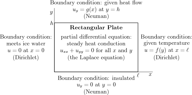
An example problem is shown in figure 1.1. Physically it is steady heat conduction in a rectangular plate of dimensions $\ell\times{h}$. The unknown $u$ in this example is the temperature. The independent variables are the Cartesian coordinates $x$ and $y$. The domain $\Omega$ is the two-dimensional interior of the plate. The boundary $\delta\Omega$ is the one-dimensional perimeter of the plate. (The boundary might still be indicated by $S$ instead of $\delta\Omega$ even though here it is not a surface.)

The Laplace equation also describes ideal flows, unidirectional flows, membranes, electrostatics and magnetostatics, complex functions, and countless other problems.

In any number of dimensions, the Laplace equation reads

$$\fbox{$\displaystyle \mbox{Laplace equation:} \qquad \nabla^2 u = 0 $} %$$ (1.1)

In particular, in three dimensions and Cartesian coordinates

$$u_{xx} + u_{yy} + u_{zz} = 0$$

For coordinates that are not Cartesian, the Laplacian $\nabla^2$ can be found in table books.

Some important properties of the Laplace equation are:

• Steady state problems: The Laplace equation normally describes processes that are in a steady state situation.
• Boundary-value problems: The Laplace equation needs “boundary-value problems.” At every point on the boundary, one boundary condition should be prescribed. For example, consider the example problem figure 1.1. On the vertical boundaries, the temperature is given. That is a Dirichlet boundary condition. On the horizontal boundaries, the heat flow out of the boundary is given. Now the heat flow is proportional to the gradient of the temperature. In particular, the heat flow in the vertical direction is proportional to $u_y$. So the horizontal boundaries have Neumann boundary conditions; the derivative of $u$ in the direction normal to these boundary is given.
• Infinite propagation speed: Sometimes the solution of the Laplace equation may still depend parametrically on time. For example, the Laplace equation applies to unsteady ideal flows of incompressible fluids. The reason that the Laplace equation can apply to such flows is that the incompressibility assumption implies an infinite speed of sound. If the boundary conditions are somewhere changed, the flow field instantly adapts to the new conditions everywhere.
• Unlimited region of influence: The Laplace equation has an unlimited region of influence. In terms of the example that means that if you change the temperature a bit somewhere on the boundary, it will affect the temperature to some extent everywhere inside the plate.
• Smoothness: The solutions to the Laplace equation are smooth. Even if you prescribe singular values for the solution on the boundary, the solution is still perfectly smooth in the interior of the domain. In particular, any point in the interior has infinitely many continuous derivatives, as well as a Taylor series with a finite radius of convergence. {D.1}
• Maximum-minimum principle: The Laplace equation has the property that the maximum and minimum of $u$ always occur on the boundary. For example, in the problem figure 1.1 the temperature in the interior of the plate can nowhere be higher than the highest temperature on the boundary. {D.2}
• Mean value theorem: Suppose $u$ is defined on and within some spherical surface and satisfies the Laplace equation. Then the average of $u$ on the spherical surface is the same as the value of $u$ at the center of the sphere. {D.2}

(For domains that extent to infinity, various rules above assume that you consider the infinite domain as the limit of a finite one.)

The Laplace equation is the basic example of what is called an “elliptic” partial differential equation. Solutions of the Laplace equation are called “harmonic functions.”

1.2.1 Review Questions

1

Derive the Laplace equation for steady heat conduction in a two-dimensional plate of constant thickness $\delta$. Do so by considering a little Cartesian rectangle of dimensions ${\Delta}x\times{\Delta}y$. A sketch is shown below:

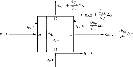
Assume Fourier’s law:

$$\vec q = (q_x,q_y) \qquad q_x = - k \frac{\partial u}{\partial x} \qquad q_y = - k \frac{\partial u}{\partial y}$$

Here $u$ is the temperature, assumed independent of $z$. Also, $k$ is the heat conduction coefficient of the material. The vector $\vec{q}$ is the heat flux density. Vector $\vec q$ is in the direction of the heat flow. Its magnitude $\vert\vec{q}\vert$ equals the heat flowing per unit area normal to the direction of flow.

If you want the heat flow $\dot Q$ through an area element ${\rm d}{S}$ that is not normal to the direction of heat flow, the expression is

$$\dot Q = \vec q \cdot{\vec n}{ \rm d}s$$

Here ${\vec n}$ is the unit vector normal to the surface element ${\rm d}{S}$. Positive $\dot{Q}$ means a heat flow through the surface element in the same direction as ${\vec n}$.

Assume that no heat is added to the little rectangle from external sources.

Solution stanexl-a

2

Derive the Laplace equation for steady heat conduction using vector analysis. Assume Fourier’s law as given in the previous question. In vector form

$$\vec q = - k \nabla u$$

Assume that no heat is added to the solid from external sources.

Solution stanexl-b

3

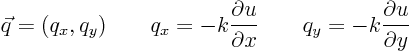
Consider the Laplace equation within a unit circle:

$$u_{xx} + u_{yy} = 0 \qquad\mbox{for}\qquad x^2+y^2<1$$

The boundary condition on the perimeter of the circle is

$$u = (y^2 + 1) x \qquad\mbox{for}\qquad x^2+y^2=1$$

To find the value of $u$ at the point (0.1,0.2), can I just plug in the coordinates of that point into the boundary condition?

There is a symmetry argument that you can give to show that $u$ is zero on the entire $y$-axis $x=0$. What?

Solution stanexl-b1

4

Consider the Laplace equation within a unit circle:

$$u_{xx} + u_{yy} = 0 \qquad\mbox{for}\qquad x^2+y^2<1$$

The boundary condition on the perimeter of the circle is

$$u = 2 + 3x + 5 y \qquad\mbox{for}\qquad x^2+y^2=1$$

Find the value of $u$ at the point (0.1,0.2). Fully defend your solution.

Solution stanexl-b2

5

Consider the Laplace equation within a unit circle, but now in polar coordinates:

$$u_{rr} + \frac 1r u_r + \frac 1{r^2} u_{\theta\theta} = 0 \qquad\mbox{for}\qquad r<1$$

The boundary condition on the perimeter of the circle is

$$u(1,\theta) = f(\theta)$$

where $f$ is a given function.

The solution is the Poisson integral formula

$$u(r,\theta) = \frac{1-r^2}{2\pi} \oint\frac{f(\bar\theta){ \rm d}\bar\theta}{1-2r\cos(\bar\theta -\theta)+r^2}$$

Now suppose that function $f(\theta)$ is increased slightly, by an amount $\delta{f}$, and only in a very small interval $\theta_1<\theta <\theta_2$.

Does the solution $u$ change everywhere in the circle, or only in the immediate vicinity of the interval on the boundary at which $f$ was changed. What is the sign of the change in $u$ if $\delta{f}$ is positive?

Solution stanexl-b3

6

• Show that if $u$ is a harmonic function in a finite domain, and positive on the boundary, then it is positive everywhere in the domain.
• Show by example that this does not need to be true for an infinite domain.
• Let $u$, $v$, and $w$ be harmonic functions. Show that if $u\le{v}\le{w}$ on the boundary of a finite domain, then $u\le{v}\le{w}$ everywhere inside the domain.

Solution stanexl-b5

7

Consider the following Laplace equation problem in a unit square:

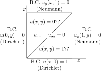
The problem as shown has a unique solution. It is relevant to a case of heat conduction in a square plate, with $u$ the temperature. Someone proposed that the solution should be simple: in the upper triangle the solution $u(x,t)$ is 0, and in the lower triangle, it is 1.

Thoroughly discuss this proposed solution. Find out whether the boundary conditions and initial conditions are satisfied. Is the partial differential equation satisfied in both triangles?

Explain why all isotherms except 0 and 1 coincide with the 45$\DG9/$ line. And why the zero and 1 isotherms are indeterminate.

Finally discuss whether the solution is right.

Solution stanexl-c

8

If the problem of the previous question does not have the proposed solution, then the isotherms are not right either.

Consider the following simpler problem, in which the top and right boundaries have been distorted into a quarter circle:

$$\mbox{BC:}\quad u(x,0)=1\quad\quad u(0,y)=0 \quad\quad\frac{\partial u}{\partial n}=0\mbox{ on }x^2+y^2=1$$

Solve this problem. Then neatly draw the $u=0$, 0.25, 0.5, 0.75, and 1 isotherms for this problem.

Also neatly draw $u$ versus the polar angle $\theta$ at $r=0.5$. In a separate graph, draw the solution proposed in the previous section, $u=1$ for $y<x$ and $u=0$ for $y>x$, again against $\theta$ at $r=0.5$.

Now go back to the problem of the previous question and very neatly sketch the correct $u=0$, 0.25, 0.5, 0.75, and 1 isotherms for that problem. Pay particular attention to where the 0.25, 0.5, and 0.75 isotherms meet the boundaries and under what angle.

Solution stanexl-d

9

Return once again to the problem of the second-last question.

The correct solution to this problem, that you would find using the so-called method of separation of variables, is:

$$u(x,y) = \sum_{\textstyle{n=1\atop n {\rm odd}}}^\infty\fra... ...tyle\frac{1}{2}}n\pi x)\cosh({\textstyle\frac{1}{2}}n\pi(1-y))$$

Verify that this solutions satisfies both the partial differential equation and all boundary conditions.

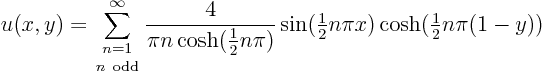
Now shed some light on the question why this solution is smooth for any arbitrary $y>0$. To do so, first explain why any sum of sines of the form

$$f(x)=\sum_{n=1}^\infty c_n \sin\left({\textstyle\frac{1}{2}}n\pi x\right)$$

is smooth as long as the sum is finite. A finite sum means that the coefficients $c_n$ are zero beyond some maximum value of $n$.

Next, you are allowed to make use of the fact that the function is still smooth if the coefficients $c_n$ go to zero quickly enough. In particular, if you can show that

$$\lim_{n\to\infty} n^k c_n = 0$$

for every $k$, however large, then the function $f(x)$ is infinitely smooth.

Use this to show that $u$ above is indeed infinitely smooth for any $y>0$. And show that it is not true for $y=0$, where the solution jumps at the origin.

Solution stanexl-e

1.2.2 The heat equation

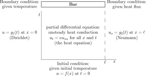
The heat equation governs basic unsteady heat conduction, among much else.

Figure 1.2: An example heat equation problem.

An example problem is shown in figure 1.2. Physically it is unsteady heat conduction in a bar of length $\ell$. The unknown $u$ is the temperature. The independent variables in this case are the coordinate $x$ along the bar and the time $t$. The domain $\Omega$ in this example is the bar. Mathematically, that is the line segment $0\le{x}\le\ell$ with $\ell$ the length of the bar. The boundary $\delta\Omega$ consists in this case of a mere two points: $x=0$ and $x=\ell$.

The heat equation also describes unsteady viscous unidirectional flows and many other diffusive phenomena.

In any number of dimensions, the heat equation reads

$$\fbox{$\displaystyle \mbox{Heat equation:} \qquad u_t = \kappa \nabla^2 u $} %$$ (1.2)

Here $t$ is time and $\kappa$ the heat conduction constant. In particular, in three dimensions and Cartesian coordinates

$$u_t = \kappa\left(u_{xx} + u_{yy} + u_{zz}\right)$$

Some important properties of the heat equation are:

• Transient problems: The heat equation normally describes processes that evolve in time.
• Initial-value or initial/boundary-value problems: The heat equation needs initial-value problems or initial/boundary-value problems. The example figure 1.2 is an initial/boundary-value problem. The initial temperature is given. In addition, there is a Dirichlet boundary condition, (given temperature $T_0$), at $x=0$. There is also a Neumann boundary condition, (zero heat flux out of the boundary so $u_x=0$), at $x=\ell$. If you let the ends of the bar go to infinity, you get a pure initial-value problem. (However, in reality there are still some constraints at infinity. In particular the temperature should not become too singular at infinity.)
• Infinite propagation speed: If you change the initial temperature or the boundary temperature a bit, it immediately changes the solution everywhere. More precisely, at any time after the change, the temperature will be different everywhere. Very little different maybe, but different.
• The region of influence is limited by time: If the boundary conditions are changed, it only changes the solution at later times.
• Smoothness: The solutions are smooth. Even if you prescribe a singular initial temperature distribution, the solution will be smooth for all later times. In particular, for later times the temperature distribution will have infinitely many continuous derivatives. A similar observation holds for boundary conditions.
• Maximum-minimum principle: The maximum and minimum of the solution must occur initially and/or on the boundaries.
• Dissipative: Assuming that the boundary conditions are steady, the solution will eventually approach a steady state.

The heat equation is the basic example of what is called a “parabolic” partial differential equation.

1.2.2 Review Questions

1

This is a continuation of a corresponding question in the subsection on the Laplace equation. See there for a definition of terms.

Derive the heat equation for unsteady heat conduction in a two-dimensional plate of thickness $\delta$, Do so by considering a little Cartesian rectangle of dimensions ${\Delta}x\times{\Delta}y$.

In particular, derive the heat conduction coefficient $\kappa$ in terms of the material heat coefficient $k$, the plate thickness $t$, and the specific heat of the solid $C_p$.

Solution stanexh-a

2

This is a continuation of a corresponding question in the subsection on the Laplace equation. See there for a definition of terms.

Derive the heat equation for unsteady heat conduction using vector analysis.

Solution stanexh-b

1.2.3 The wave equation

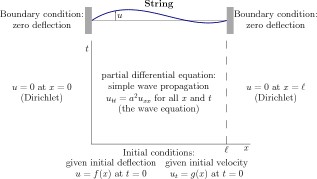
This equation governs basic vibrations, among much else.

Figure 1.3: An example wave equation problem.

An example problem, vibrations of a string, is shown in figure 1.3. The unknown $u$ is the transverse deflection of the string. The independent variables are again $x$ and $t$ like for the heat equation example. The domain $\Omega$ is again the $x$-interval along the string and the boundary $\delta\Omega$ is the two end points.

The heat equation also describes acoustics, steady supersonic flow, water waves, optics, electromagnetic waves, and many other basic phenomena characterized by wave propagation.

In any number of dimensions, the wave equation reads

$$\fbox{$\displaystyle \mbox{Wave equation:} \qquad u_{tt} = a^2 \nabla^2 u $} %$$ (1.3)

Here $t$ is time and $a$ the constant wave propagation speed. In particular, in three dimensions and Cartesian coordinates

$$u_{tt} = a^2\left(u_{xx} + u_{yy} + u_{zz}\right)$$

Some important properties of the wave equation are:

• Transient problems: The wave equation normally describes processes that evolve in time.
• Initial-value or initial/boundary-value problems: Like the heat equation, the wave equation needs initial-value problems or initial/boundary-value problems. However, it needs two initial conditions instead of one, since the equation is second order in time. For the example figure 1.2, that means that both the initial transverse deflection $u$ and the initial transverse velocity $u_t$ of each point of the string must be given. A string would normally be fixed at its end points, producing Dirichlet boundary conditions. However, the same equation as in the example also governs acoustics in a pipe, and either Dirichlet or Neumann boundary conditions may be relevant to the ends of the pipe.
• Finite propagation speed: Effects propagate with the wave speed $a$.
• The region of influence is limited by the wave speed: Suppose that a boundary or initial condition is somewhere changed a bit. The change will not affect the solution at other locations until a wave traveling from the point of the change at speed $a$ has had time to reach them.
• Propagation of singularities: If singular initial or boundary conditions are prescribed, the wave equation will not smooth them out. Instead singularities will usually be propagated in one or more directions with the wave propagation speed $a$.
• No maximum or minimum principles: For the example, if the string has zero initial deflection but a nonzero initial velocity, the deflection will grow in time.
• Energy conservation: The wave equation preserves the sum of potential and kinetic energy of the string motion. So, if the wave equation was exact, the string would keep vibrating forever.

The wave equation is the basic example of what is called a “hyperbolic” partial differential equation.

1.2.3 Review Questions

1

Derive the wave equation for small transverse vibrations of a string by considering a little string segment of length ${\Delta}x$.

Solution stanexw-a

2

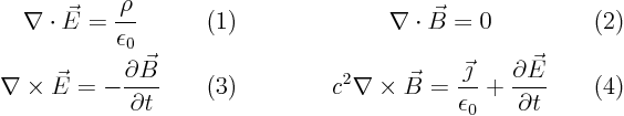
Maxwell’s equations for the electromagnetic field in vacuum are

$$\begin{array}{ccccc} \displaystyle\nabla\cdot\vec E = \frac{... ...on_0} +\frac{\partial\vec E}{\partial t} & \quad(4) \end{array}$$

Here $\vec{E}$ is the electric field, $\vec{B}$ the magnetic field, $\rho$ the charge density, $\vec\jmath$ the current density, $c$ the constant speed of light, and $\epsilon_0$ is a constant called the permittivity of space. The charge and current densities are related by the continuity equation

$$\frac{\partial\rho}{\partial t} + \nabla\cdot\vec\jmath = 0 \qquad(5)$$

Show that if you know how to solve the standard wave equation, you know how to solve Maxwell’s equations. At least, if the charge and current densities are known.

Identify the wave speed.

Solution stanexw-b

3

Consider the following wave equation problem in a unit square:

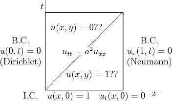
This is basically identical to a Laplace equation problem in the first subsection. Like that problem, the above wave equation problem has a unique solution. It is relevant to a case of acoustics in a tube, with $u$ the pressure. Someone proposed that the solution should be simple: in the upper triangle the solution $u(x,t)$ is 0, and in the lower triangle, it is 1.

Thoroughly discuss this proposed solution. Find out whether the boundary conditions and initial conditions are satisfied. Is the partial differential equation satisfied in both triangles? Finally discuss whether the solution is right. Consider the value of the wave speed $a$ in your answer.

Sketch the isobars of the correct solution. In particular, sketch the $u=0$ 0.25, 0.5, 0.75, and 1 isobars, if possible. Sketch both the case that $a=1$ and that $a=\sqrt{2}$.

Solution stanexw-c

4

Return again to the problem of the last question. Assume $a=1$.

The correct solution to this problem, that you would find using the so-called method of separation of variables, is:

$$u = \sum_{\textstyle{n=1\atop n {\rm odd}}}^\infty\frac{4}{... ...extstyle\frac{1}{2}}n\pi x)\cos({\textstyle\frac{1}{2}}n\pi t)$$

Verify that this solutions satisfies both the partial differential equation and all boundary and initial conditions.

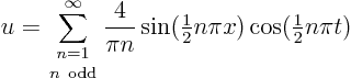
Explain that it produces the moving jump in the solution as given in the previous question.

The discontinuous solution given in the previous question is right in this case. It is right because it is the proper limiting case of a smooth solution that everywhere satisfies the partial differential equation. In particular, if you sum the above sum for $u$ up to a very high, but not infinite value of $n$, you get a smooth solution of the partial differential equation that satisfies all initial and boundary conditions, except that the value of $u$ at $t=0$ still shows small deviations from $u=1$. The more terms you sum, the smaller those deviations become. (There will always be some differences right at the singularity, but these will be restricted to a negligibly small vicinity of $x=0$.)

Solution stanexw-e

5

Find the possible plane wave solutions for the two-dimensional wave equation

$$u_{tt} = a^2 u_{xx} + a^2 u_{yy}$$

What is the wave speed?

Also find the possible standing wave solutions. Assume homogeneous Dirichlet or Neumann boundary conditions on some rectangle $0<x<\ell$, $0<y<h$. What is the frequency?

Repeat for the generalized equation

$$u_{tt} = a_1^2 u_{xx} + a_2^2 u_{yy} + b^2 u$$

where $a_1$, $a_2$, and $b$ are positive constants.

Solution stanexw-f