1.3 Classification

1.3.1 Introduction

Classification groups partial differential equations with similar properties together.

One set of partial differential equations that has a unambiguous classification are 2D second order quasi-linear equations:

$$a u_{xx} + 2 b u_{xy} + c u_{yy} = d$$

where $a=a(x,y,u,u_x,u_y)$, $b=b(x,y,u,u_x,u_y)$, $c=c(x,y,u,u_x,u_y)$, and $d=d(x,y,u,u_x,u_y)$.

The classification for these equations is:

• $b^2 - ac > 0$: hyperbolic
• $b^2 - ac = 0$: parabolic
• $b^2 - ac < 0$: elliptic

Example

Question: Classify the equation

$$y u_{xx} -2 u_{xy} + e^x u_{yy} + u = 3$$

Solution:

Identify the coefficients and find the discriminant:

$$a = y, b = -1, c= e^x \quad\quad\Rightarrow\quad\quad b^2 - ac = 1 - y e^x$$

So it is parabolic for

$$1 - y e^x = 0 \quad\quad\Rightarrow\quad\quad y = e^{-x},$$

It is elliptic if $y$ is greater than the value above and hyperbolic if $y$ is less.

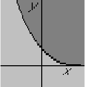
Graphically:

$$\hbox{\epsffile{2dcl.eps}}$$

Example

Question: Classify the potential equation for compressible flow for an airfoil:

$$(a^2-\phi_x^2)\phi_{xx} - -2\phi_x\phi_y\phi_{xy} + (a^2-\phi_y^2)\phi_{xx} = 0$$

Here $a$ is the speed of sound, not to be confused with the $a$ in the generic partial differential equation. Also $\phi_x$ and $\phi_y$ are the velocity components $u$ and $v$ in the $x$ and $y$ directions. Discuss the associated physics.

Solution:

The discriminant is

$$(\phi_x\phi_y)^2 - (a^2-\phi_x^2)(a^2-\phi_y^2)$$

or in terms of velocity and speed of sound:

$$u^2v^2 - (a^2-u^2)(a^2-v^2)$$

Multiplying out gives

$$a^2[a^2-(u^2+v^2)]$$

Note that the term within square brackets is positive if the magnitude of the speed of sound is greater than the magnitude of the velocity. That is subsonic flow, with a Mach number

$$M = \frac{\sqrt{u^2+v^2}}{a}$$

less than 1. The equation is then elliptic. Conversely, if the flow velocity is greater than the speed of sound, supersonic flow, then the equation is hyperbolic.

Consider a picture of transonic flow around an airfoil:

$$\hbox{\epsffile{airfoil.eps}}$$

The subsonic region does indeed behave elliptic. There are smooth solutions and an unlimited region of dependence. Numerically, this region must be solved through simultaneous global solution.

The supersonic region behaves hyperbolic. There are singularities like expansion fans and shocks. The propagation of Mach lines is given by the so-called Mach-angle. The solution can numerically be found station by station using a marching scheme.

1.3.2 Scalar second order equations

The general $n$-dimensional second order quasi-linear second order equation is:

$$\begin{array}{ccccccccc} a_{11} u_{x_1x_1} &+& a_{12} u_... ...\ \vdots && \vdots && \vdots && \ddots &=& d \end{array}$$

The coefficients are not quite unique: since the order of differentiation can be reversed, a coefficient like $a_{12}$ is equivalent to $a_{21}$. The coefficients will be made unique by requiring that they form a symmetric matrix $A$. That means, for example, that $a_{12}=a_{21}$.

In index notation, the n-dimensional equation can then be written as:

$$\fbox{$\displaystyle \sum_i \sum_j a_{ij} \frac{\partial^2 u}{\partial x_i \partial x_j} = d $} %$$ (1.4)

where the coefficients $a_{ij}=a_{ij}(x_1,x_2,\ldots,x_n,u,u_{x_1},u_{x_2},\ldots,u_{x_n})$ form a symmetric matrix $A$ and $d=d(x_1,x_2,\ldots,x_n,u,u_{x_1},u_{x_2},\ldots,u_{x_n})$.

Example

Question: Find matrix $A$ for the generic two-dimensional equation

$$a u_{xx}+ 2 b u_{xy} + c u_{yy} = d$$

Solution: Writing the equation in $n$-dimensional form gives:

$$a_{11} u_{xx}+ a_{12} u_{xy} +a_{21} u_{xy} + a_{22} u_{yy} = d$$

Comparing with the equation above, $a_{11}=a$, $a_{12}=a_{21}=b$, and $a_{22}=c$. So the matrix $A$ is here:

$$A = \left( \begin{array}{cc} a & b \\ b & c \end{array} \right)$$

Classification is based on the eigenvalues of $A$:

• parabolic if any eigenvalues are zero; otherwise:
• elliptic if all eigenvalues are the same sign;
• hyperbolic if all eigenvalues except one are of the same sign;
• ultrahyperbolic, otherwise.

The reason for this classification will be explained later, in section 1.4.4.

Example

Question: Figure out why that is consistent with what we defined for the two-dimensional case,

$$A = \left( \begin{array}{cc} a & b \\ b & c \en... ... \\ \mbox{elliptic if $b^2-ac<0$} \end{array} \right.$$

Solution: From linear algebra it is known that the determinant of a matrix equals the product of its eigenvalues. In this case there are two eigenvalues. Their product is the determinant:

$$\lambda_1 \lambda_2 = \left\vert \begin{array}{cc} a & b \\ b & c \end{array} \right\vert = ac - b^2$$

According to the $n$-dimensional classification scheme, the equation is parabolic if an eigenvalue is zero. But then the product $ac-b^2$ of the eigenvalues will be zero. So $b^2-ac$ is zero too, and that also makes the equation parabolic according to the two-dimensional classification scheme.

According to the $n$-dimensional classification scheme, the equation is elliptic when the two eigenvalues are of the same sign. But then the product of the eigenvalues is positive, $ac-b^2>0$. That makes $b^2-ac$ negative in agreement with the two-dimensional classification.

The only remaining possibility is that the eigenvalues are of opposite sign. That makes their product $ac-b^2$ negative, again in agreement with the two-dimensional classification.

Example

Question:

$$\hbox{\epsffile{ndcl.eps}}$$

The equation

$$u_t - \nabla \cdot (p \nabla u) + q u = f$$

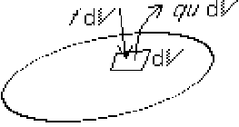
is a generic unsteady heat conduction equation, with $u$ the temperature relative to the surroundings. The first term is the rate of temperature change at a point. The second term represents heat accumulation due to conduction of heat. In it, $p$ is the heat conduction coefficient. The third term would in two dimensions be an approximation to the heat radiated away to the surroundings. The right hand side represents heat that is explicitly added from other sources. Classify this equation.

Solution: Write out the equation using the definition of nabla:

$$\nabla = {\hat\imath}\frac{\partial}{\partial x} + {\h... ...partial}{\partial y} + {\hat k}\frac{\partial}{\partial z}$$

Then

$$\nabla u \equiv \hbox{grad } u = {\hat\imath}u_x + {\hat\jmath}u_y + {\hat k}u_z$$

$$\nabla \cdot \vec v \equiv \hbox{div } \vec v = v_{1x} + v_{2y} + v_{3z}$$

The equation is therefore

$$u_t - (p u_x)_x - (p u_y)_y - (p u_z)_z + q u = f$$

Now identify the highest derivatives of $u$:

$$- p u_{xx} - p u_{yy} - p u_{zz} + \ldots = f$$

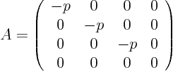
Find the coefficient matrix $A$

$$A = \left( \begin{array}{cccc} -p& 0 & 0 & 0 \\ 0... ... 0 & 0 & -p& 0 \\ 0 & 0 & 0 & 0 \end{array} \right)$$

The eigenvalues are $\lambda_1 =\lambda_2 =\lambda_3 = -p$ and $\lambda_4 = 0$. The zero eigenvalue makes it parabolic.

Note that the equation is a partial differential equation in four dimensions even though there are no second order derivatives involving time. There is still a first order time derivative.

1.3.2 Review Questions

1

Classify the equations

$$u_{tt} - \nabla\cdot(p \nabla u) + q u = f \qquad - \nabla\cdot(p \nabla u) + q u = f$$

Solution clasnd-a