How you treat a substance depends on the type of substance.
Tables of specific properties such as tables B.1.1-B.1.4 for water are
available. Use requires normally drawing ![]() - and
- and ![]() - or
- or
![]() -diagrams, which students must master, and which is covered
elsewhere.
-diagrams, which students must master, and which is covered
elsewhere.
In the two phase region:
For compressed liquids, often there are no suitable tables available.
Fortunately, good approximate values for ![]() ,
, ![]() ,
, ![]() , and
, and ![]() can
usually be taken from the saturated tables at the correct given
temperature. The fact that the given pressure is not the same as the
saturated pressure must then be ignored. (For
can
usually be taken from the saturated tables at the correct given
temperature. The fact that the given pressure is not the same as the
saturated pressure must then be ignored. (For ![]() , it is more
accurate to write
, it is more
accurate to write ![]() and then take
and then take ![]() and
and ![]() from the
saturated tables, instead of
from the
saturated tables, instead of ![]() itself.)
itself.)
Specific gas constant ![]() in terms of the universal gas constant
in terms of the universal gas constant ![]() (table A.1):
(table A.1):
Forms of the ideal gas law:

To correct for real gas effects, replace ![]() (or
(or ![]() ) by
) by ![]() (
(![]() ), where
), where ![]() is the compressibility factor (figure D1, with
is the compressibility factor (figure D1, with
![]() ,
, ![]() .)
.)
For an ideal gas, ![]() ,
, ![]() ,
, ![]() ,
, ![]() , and
, and ![]() only depend on
temperature. Also,
only depend on
temperature. Also,
Specific heat relation:
Definition of specific heat ratio:
Note that isothermal ideal gasses are also polytropic with ![]() .
.
The internal energy ![]() and enthalpy
and enthalpy ![]() can be read off in the table
as a function of temperature. Or vice-versa, for that matter.
can be read off in the table
as a function of temperature. Or vice-versa, for that matter.
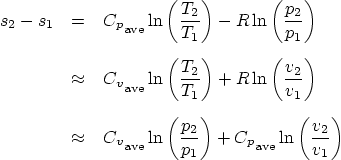
The formula that gives you the entropy ![]() is, (in terms of differences),
is, (in terms of differences),
If no A.7.1/A.8 table is available, you will have to assume that the
specific heats ![]() and
and ![]() , as well as their ration
, as well as their ration ![]() are
constant. Specific heats that can be assumed to be approximately
constant can be computed from the average process temperature using
table A.6. Less accurately, near room temperature they can be taken
from A.5. Use A.6 wherever possible unless you are very close to
room temperature.
are
constant. Specific heats that can be assumed to be approximately
constant can be computed from the average process temperature using
table A.6. Less accurately, near room temperature they can be taken
from A.5. Use A.6 wherever possible unless you are very close to
room temperature.
Internal energy:
Enthalpy:
Entropy:

If the process is isothermal or reversible adiabatic (isentropic), the
following “polytropic” relations also apply (they are
equivalent to the equations above, but often much more convenient):

Approximate formulae if no better tabulated values are available, or to simplify things.
Heat added:
Enthalpy:
Entropy: