7.2 Time Vari­a­tion of Ex­pec­ta­tion Val­ues

The time evo­lu­tion of sys­tems may be found us­ing the Schrö­din­ger equa­tion as de­scribed in the pre­vi­ous sec­tion. How­ever, that re­quires the en­ergy eigen­func­tions to be found. That might not be easy.

For some sys­tems, es­pe­cially for macro­scopic ones, it may be suf­fi­cient to fig­ure out the evo­lu­tion of the ex­pec­ta­tion val­ues. An ex­pec­ta­tion value of a phys­i­cal quan­tity is the av­er­age of the pos­si­ble val­ues of that quan­tity, chap­ter 4.4. This sec­tion will show how ex­pec­ta­tion val­ues may of­ten be found with­out find­ing the en­ergy eigen­func­tions. Some ap­pli­ca­tions will be in­di­cated.

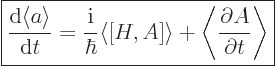
The Schrö­din­ger equa­tion re­quires that the ex­pec­ta­tion value $\left\langle{a}\right\rangle$ of any phys­i­cal quan­tity $a$ with as­so­ci­ated op­er­a­tor $A$ evolves in time as:

$$\fbox{$\displaystyle \frac{{\rm d}\langle a \rangle}{{\rm ... ...\left\langle \frac{\partial A}{\partial t} \right\rangle $} %$$ (7.4)

A de­riva­tion is in {D.35}. The com­mu­ta­tor $[H,A]$ of $A$ with the Hamil­ton­ian was de­fined in chap­ter 4.5 as $HA-AH$. The fi­nal term in (7.4) is usu­ally zero, since most (sim­ple) op­er­a­tors do not ex­plic­itly de­pend on time.

The above evo­lu­tion equa­tion for ex­pec­ta­tion val­ues does not re­quire the en­ergy eigen­func­tions, but it does re­quire the com­mu­ta­tor.

Note from (7.4) that if an op­er­a­tor $A$ com­mutes with the Hamil­ton­ian, i.e. $[H,A]$ $\vphantom0\raisebox{1.5pt}{$=$}$ 0, then the ex­pec­ta­tion value of the cor­re­spond­ing quan­tity $a$ will not vary with time. Ac­tu­ally, that is just the start of it. Such a quan­tity has eigen­func­tions that are also en­ergy eigen­func­tions, so it has the same time-con­served sta­tis­tics as en­ergy, sec­tion 7.1.4. The un­cer­tainty, prob­a­bil­i­ties of the in­di­vid­ual val­ues, etcetera, do not change with time ei­ther for such a vari­able.

One ap­pli­ca­tion of equa­tion (7.4) is the so-called “vir­ial the­o­rem” that re­lates the ex­pec­ta­tion po­ten­tial and ki­netic en­er­gies of en­ergy eigen­states, {A.17}. For ex­am­ple, it shows that har­monic os­cil­la­tor states have equal po­ten­tial and ki­netic en­er­gies. And that for hy­dro­gen states, the po­ten­tial en­ergy is mi­nus two times the ki­netic en­ergy.

Two other im­por­tant ap­pli­ca­tions are dis­cussed in the next two sub­sec­tions.

Key Points

$\begin{picture}(15,5.5)(0,-3) \put(2,0){\makebox(0,0){\scriptsize\bf0}} \put(12... ...\thicklines \put(3,0){\line(1,0){12}}\put(11.5,-2){\line(1,0){3}} \end{picture}$

A rel­a­tively sim­ple equa­tion that de­scribes the time evo­lu­tion of ex­pec­ta­tion val­ues of phys­i­cal quan­ti­ties ex­ists. It is fully in terms of ex­pec­ta­tion val­ues.

$\begin{picture}(15,5.5)(0,-3) \put(2,0){\makebox(0,0){\scriptsize\bf0}} \put(12... ...\thicklines \put(3,0){\line(1,0){12}}\put(11.5,-2){\line(1,0){3}} \end{picture}$

Vari­ables which com­mute with the Hamil­ton­ian have the same time-in­de­pen­dent sta­tis­tics as en­ergy.

$\begin{picture}(15,5.5)(0,-3) \put(2,0){\makebox(0,0){\scriptsize\bf0}} \put(12... ...\thicklines \put(3,0){\line(1,0){12}}\put(11.5,-2){\line(1,0){3}} \end{picture}$

The vir­ial the­o­rem re­lates the ex­pec­ta­tion ki­netic and po­ten­tial en­er­gies for im­por­tant sys­tems.

7.2.1 New­ton­ian mo­tion

The pur­pose of this sec­tion is to show that even though New­ton's equa­tions do not ap­ply to very small sys­tems, they are cor­rect for macro­scopic sys­tems.

The trick is to note that for a macro­scopic par­ti­cle, the po­si­tion and mo­men­tum are very pre­cisely de­fined. Many un­avoid­able phys­i­cal ef­fects, such as in­ci­dent light, col­lid­ing air atoms, ear­lier his­tory, etcetera, will nar­row down po­si­tion and mo­men­tum of a macro­scopic par­ti­cle to great ac­cu­racy. Heisen­berg's un­cer­tainty re­la­tion­ship says that they must have un­cer­tain­ties big enough that $\Delta{p}_x\Delta{x}$ $\raisebox{-.5pt}{$\geqslant$}$ $\frac12\hbar$, but $\hbar$ is far too small for that to be no­tice­able on a macro­scopic scale. Nor­mal light changes the mo­men­tum of a rocket ship in space only im­mea­sur­ably lit­tle, but it is quite ca­pa­ble of lo­cat­ing it to ex­cel­lent ac­cu­racy.

With lit­tle un­cer­tainty in po­si­tion and mo­men­tum, both can be ap­prox­i­mated ac­cu­rately by their ex­pec­ta­tion val­ues. So the evo­lu­tion of macro­scopic sys­tems can be ob­tained from the evo­lu­tion equa­tion (7.4) for ex­pec­ta­tion val­ues given in the pre­vi­ous sub­sec­tion. Just work out the com­mu­ta­tor that ap­pears in it.

Con­sider one-di­men­sion­al mo­tion of a par­ti­cle in a po­ten­tial $V(x)$ (the three-di­men­sion­al case goes ex­actly the same way). The Hamil­ton­ian $H$ is:

$$H = \frac{{\widehat p}_x^2}{2m} + V(x)$$

where ${\widehat p}_x$ is the lin­ear mo­men­tum op­er­a­tor and $m$ the mass of the par­ti­cle.

Now ac­cord­ing to evo­lu­tion equa­tion (7.4), the ex­pec­ta­tion po­si­tion $\left\langle{x}\right\rangle$ changes at a rate:

$$\frac{{\rm d}\langle x \rangle}{{\rm d}t} = \left\langle \... ...{\widehat p}_x^2}{2m} + V(x),{\widehat x}\right] \right\rangle$$ (7.5)

Re­call­ing the prop­er­ties of the com­mu­ta­tor from chap­ter 4.5, $[V(x),{\widehat x}]$ $\vphantom0\raisebox{1.5pt}{$=$}$ 0, since mul­ti­pli­ca­tion com­mutes. Fur­ther, ac­cord­ing to the rules for ma­nip­u­la­tion of prod­ucts and the canon­i­cal com­mu­ta­tor

$$[{\widehat p}_x^2,{\widehat x}]= {\widehat p}_x[{\widehat p}_... ...\widehat p}_x]{\widehat p}_x = - 2 {\rm i}\hbar {\widehat p}_x$$

So the rate of change of ex­pec­ta­tion po­si­tion be­comes:

$$\frac{{\rm d}\langle x \rangle}{{\rm d}t} = \left\langle \frac{p_x}{m} \right\rangle$$ (7.6)

This is ex­actly the New­ton­ian ex­pres­sion for the change in po­si­tion with time, be­cause New­ton­ian me­chan­ics de­fines $p_x$$\raisebox{.5pt}{$/$}$​$m$ to be the ve­loc­ity. How­ever, it is in terms of ex­pec­ta­tion val­ues.

To fig­ure out how the ex­pec­ta­tion value of mo­men­tum varies, the com­mu­ta­tor $[H,{\widehat p}_x]$ is needed. Now ${\widehat p}_x$ com­mutes, of course, with it­self, but just like it does not com­mute with ${\widehat x}$, it does not com­mute with the po­ten­tial en­ergy $V(x)$. The gen­er­al­ized canon­i­cal com­mu­ta­tor (4.62) says that $[V,{\widehat p}_x]$ equals $\vphantom{0}\raisebox{1.5pt}{$-$}$$\hbar\partial{V}$$\raisebox{.5pt}{$/$}$​${\rm i}\partial{x}$. As a re­sult, the rate of change of the ex­pec­ta­tion value of lin­ear mo­men­tum be­comes:

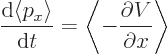$$\frac{{\rm d}\langle p_x \rangle}{{\rm d}t} = \left\langle - \frac{\partial V}{\partial x} \right\rangle$$ (7.7)

This is New­ton's sec­ond law in terms of ex­pec­ta­tion val­ues: New­ton­ian me­chan­ics de­fines the neg­a­tive de­riv­a­tive of the po­ten­tial en­ergy to be the force, so the right hand side is the ex­pec­ta­tion value of the force. The left hand side is equiv­a­lent to mass times ac­cel­er­a­tion.

The fact that the ex­pec­ta­tion val­ues sat­isfy the New­ton­ian equa­tions is known as “Ehren­fest's the­o­rem.”

For a quan­tum-scale sys­tem, how­ever, it should be cau­tioned that even the ex­pec­ta­tion val­ues do not truly sat­isfy New­ton­ian equa­tions. New­ton­ian equa­tions use the force at the ex­pec­ta­tion value of po­si­tion, in­stead of the ex­pec­ta­tion value of the force. If the force varies non­lin­early over the range of pos­si­ble po­si­tions, it makes a dif­fer­ence.

There is a al­ter­na­tive for­mu­la­tion of quan­tum me­chan­ics due to Heisen­berg that is like the Ehren­fest the­o­rem on steroids, {A.12}. Here the op­er­a­tors sat­isfy the New­ton­ian equa­tions.

Key Points

$\begin{picture}(15,5.5)(0,-3) \put(2,0){\makebox(0,0){\scriptsize\bf0}} \put(12... ...\thicklines \put(3,0){\line(1,0){12}}\put(11.5,-2){\line(1,0){3}} \end{picture}$

New­ton­ian physics is an ap­prox­i­mate ver­sion of quan­tum me­chan­ics for macro­scopic sys­tems.

$\begin{picture}(15,5.5)(0,-3) \put(2,0){\makebox(0,0){\scriptsize\bf0}} \put(12... ...\thicklines \put(3,0){\line(1,0){12}}\put(11.5,-2){\line(1,0){3}} \end{picture}$

The equa­tions of New­ton­ian physics ap­ply to ex­pec­ta­tion val­ues.

7.2.2 En­ergy-time un­cer­tainty re­la­tion

The Heisen­berg un­cer­tainty re­la­tion­ship pro­vides an in­tu­itive way to un­der­stand the var­i­ous weird fea­tures of quan­tum me­chan­ics. The re­la­tion­ship says $\Delta{p}_x\Delta{x}$ $\raisebox{-.5pt}{$\geqslant$}$ $\frac12\hbar$, chap­ter 4.5.3. Here $\Delta{p}_x$ is the un­cer­tainty in a com­po­nent of the mo­men­tum of a par­ti­cle, and $\Delta{x}$ is the un­cer­tainty in the cor­re­spond­ing com­po­nent of po­si­tion.

Now spe­cial rel­a­tiv­ity con­sid­ers the en­ergy $E$ di­vided by the speed of light $c$ to be much like a ze­roth mo­men­tum co­or­di­nate, and $ct$ to be much like a ze­roth po­si­tion co­or­di­nate, chap­ter 1.2.4 and 1.3.1. Mak­ing such sub­sti­tu­tions trans­forms Heisen­berg’s re­la­tion­ship into the so-called “en­ergy-time un­cer­tainty re­la­tion­ship:”

$$\fbox{$\displaystyle \Delta E\; \Delta t\mathrel{\raisebox{-1pt}{$\geqslant$}}\frac12\hbar $} %$$ (7.8)

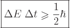
There is a dif­fer­ence, how­ever. In Heisen­berg’s orig­i­nal re­la­tion­ship, the un­cer­tain­ties in mo­men­tum and po­si­tions are math­e­mat­i­cally well de­fined. In par­tic­u­lar, they are the stan­dard de­vi­a­tions in the mea­sur­able val­ues of these quan­ti­ties. The un­cer­tainty in en­ergy in the en­ergy-time un­cer­tainty re­la­tion­ship can be de­fined sim­i­larly. The prob­lem is what to make of that un­cer­tainty in time $\Delta{t}$. The Schrö­din­ger equa­tion treats time fun­da­men­tally dif­fer­ent from space.

One way to ad­dress the prob­lem is to look at the typ­i­cal evo­lu­tion time of the ex­pec­ta­tion val­ues of quan­ti­ties of in­ter­est. Us­ing care­ful an­a­lyt­i­cal ar­gu­ments along those lines, Man­delsh­tam and Tamm suc­ceeded in giv­ing a mean­ing­ful de­f­i­n­i­tion of the un­cer­tainty in time, {A.18}. Un­for­tu­nately, its use­ful­ness is lim­ited.

Ig­nore it. Care­ful an­a­lyt­i­cal ar­gu­ments are for wimps! Take out your pen and cross out $\Delta{t}$. Write in any time dif­fer­ence you want. Cross out $\Delta{E}$ and write in “any en­ergy dif­fer­ence you want.” As long as you are at it any­way, also cross out $\raisebox{-.5pt}{$\geqslant$}$” and write in “$\vphantom0\raisebox{1.5pt}{$=$}$. This can be jus­ti­fied be­cause both are math­e­mat­i­cal sym­bols. And in­equal­i­ties are so vague any­way. You have now ob­tained the pop­u­lar ver­sion of the Heisen­berg en­ergy-time un­cer­tainty equal­ity:

$$\fbox{$\displaystyle \mbox{any energy difference you want}... ...me difference you want} = {\textstyle\frac{1}{2}} \hbar $} %$$ (7.9)

This is an ex­tremely pow­er­ful equa­tion that can ex­plain any­thing in quan­tum physics in­volv­ing any two quan­ti­ties that have di­men­sions of en­ergy and time. Be sure, how­ever, to only pub­li­cize the cases in which it gives the right an­swer.

Key Points

$\begin{picture}(15,5.5)(0,-3) \put(2,0){\makebox(0,0){\scriptsize\bf0}} \put(12... ...\thicklines \put(3,0){\line(1,0){12}}\put(11.5,-2){\line(1,0){3}} \end{picture}$

The en­ergy-time un­cer­tainty re­la­tion­ship is a gen­er­al­iza­tion of the Heisen­berg un­cer­tainty re­la­tion­ship. It re­lates un­cer­tainty in en­ergy to un­cer­tainty in time. What un­cer­tainty in time means is not ob­vi­ous.

$\begin{picture}(15,5.5)(0,-3) \put(2,0){\makebox(0,0){\scriptsize\bf0}} \put(12... ...\thicklines \put(3,0){\line(1,0){12}}\put(11.5,-2){\line(1,0){3}} \end{picture}$

If you are not a wimp, the an­swer to that prob­lem is easy.