| Quantum Mechanics for Engineers |
|
© Leon van Dommelen |
|
Subsections
A.19 Conservation Laws and Symmetries
This note has a closer look at the relation between conservation laws
and symmetries. As an example it derives the law of conservation of
angular momentum directly from the rotational symmetry of physics. It
then briefly explains how the arguments carry over to other
conservation laws like linear momentum and parity. A simple example
of a local gauge symmetry is also given. The final subsection has a
few remarks about the symmetry of physics with respect to time shifts.
A.19.1 An example symmetry transformation
The mathematician Weyl gave a simple definition of a symmetry. A
symmetry exists if you do something and it does not make a difference.
A circular cylinder is an axially symmetric object because if you
rotate it around its axis over some arbitrary angle, it still looks
exactly the same. However, this note is not concerned with symmetries
of objects, but of physics. That are symmetries where you do
something, like place a system of particles at a different position or
angle, and the physics stays the same. The system of particles itself
does not necessarily need to be symmetric here.
As an example, this subsection and the next ones will explore one
particular symmetry and its conservation law. The symmetry is that
the physics is the same if a system of particles is placed under a
different angle in otherwise empty space. There are no preferred
directions in empty space. The angle that you place a system under
does not make a difference. The corresponding conservation law will
turn out to be conservation of angular momentum.
First a couple of clarifications. Empty space should really be
understood to mean that there are no external effects on the system.
A hydrogen atom in a vacuum container on earth is effectively in empty
space. Or at least it is as far as its electronic structure is
concerned. The energies associated with the gravity of earth and with
collisions with the walls of the vacuum container are negligible.
Atomic nuclei are normally effectively in empty space because the
energies to excite them are so large compared to electronic energies.
As a macroscopic example, to study the internal motion of the solar
system the rest of the galaxy can presumably safely be ignored. Then
the solar system too can be considered to be in empty space.
Further, placing a system under a different angle may be somewhat
awkward. Don’t burn your fingers on that hot sun when placing the
solar system under a different angle. And there always seems to be a
vague suspicion that you will change something nontrivially by placing
the system under a different angle.
There is a different, better, way. Note that you will always need a
coordinate system to describe the evolution of the system of particles
mathematically. Instead of putting the system of particles under an
different angle, you can put that coordinate system under a different
angle. It has the same effect. In empty space there is no reference
direction to say which one got rotated, the particle system or the
coordinate system. And rotating the coordinate system leaves the
system truly untouched. That is why the view that the coordinate
system gets rotated is called the “passive view.” The view that the system itself gets rotated is
called the “active view.”
Figure A.7:
Effect of a rotation of the coordinate system on the
spherical coordinates of a particle at an arbitrary location P.
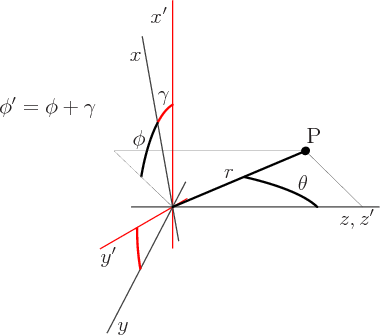 |
Figure A.7 shows graphically what happens to the
position coordinates of a particle if the coordinate system gets
rotated. The original coordinate system is indicated by primes. The
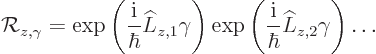
 -axis has been chosen along the axis of the desired rotation.
Rotation of this coordinate system over an angle
-axis has been chosen along the axis of the desired rotation.
Rotation of this coordinate system over an angle  produces a
new coordinate system indicated without primes. In terms of spherical
coordinates, the radial position
produces a
new coordinate system indicated without primes. In terms of spherical
coordinates, the radial position  of the particle does not change.
And neither does the
of the particle does not change.
And neither does the polar
angle  . But
the
. But
the azimuthal
angle  does change. As the figure
shows, the relation between the azimuthal angles is
does change. As the figure
shows, the relation between the azimuthal angles is
That is the basic mathematical description of the symmetry
transformation.
However, it must still be applied to the description of the physics.
And in quantum mechanics, the physics is described by a wave function
 that depends on the position coordinates of the particles;
where 1, 2, ..., is the numbering of the particles. Particle spin
will be ignored for now.
Physically absolutely nothing changes if the coordinate system is
rotated. So the values of the wave function in the
rotated coordinate system are exactly the same as the values  in the original coordinate system. But the particle coordinates
corresponding to these values do change:
in the original coordinate system. But the particle coordinates
corresponding to these values do change:
Therefore, considered as functions, and are
different. However, only the azimuthal angles change. In particular,
putting in the relation between the azimuthal angles above gives:
Mathematically, changes in functions are most conveniently written in
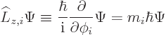
terms of an appropriate operator, chapter 2.4. The
operator here is called the “generator of rotations around the  -axis.” It will be
indicated as
-axis.” It will be
indicated as  . What it does is add to
the azimuthal angles of the function. By definition:
. What it does is add to
the azimuthal angles of the function. By definition:
In terms of this operator, the relationship between the wave functions
in the rotated and original coordinate systems can be written
concisely as
Using , there is no longer a need for using primes
on one set of coordinates. Take any wave function in terms of the
original coordinates, written without primes. Application of
will turn it into the corresponding wave function in
the rotated coordinates, also written without primes.
So far, this is all mathematics. The above expression applies whether
or not there is symmetry with respect to rotations. It even applies
whether or not is a wave function.
A.19.2 Physical description of a symmetry
The next question is what it means in terms of physics that empty
space has no preferred directions. According to quantum mechanics,
the Schrödinger equation describes the physics. It says that the
time derivative of the wave function can be found as
where  is the Hamiltonian. If space has no preferred directions,
then the Hamiltonian must be the same regardless of angular
orientation of the coordinate system used.
is the Hamiltonian. If space has no preferred directions,
then the Hamiltonian must be the same regardless of angular
orientation of the coordinate system used.
In particular, consider the two coordinate systems of the previous
subsection. The second system differed from the first by a rotation
over an arbitrary angle around the -axis. If one system
had a different Hamiltonian than the other, then systems of particles
would be observed to evolve in a different way in that coordinate
system. That would provide a fundamental distinction between the two
coordinate system orientations right there.
A couple of very basic examples can make this more concrete. Consider
the electronic structure of the hydrogen atom as analyzed in chapter
4.3. The electron was not in empty space in that
analysis. It was around a proton, which was assumed to be at rest at
the origin. However, the electric field of the proton has no
preferred direction either. (Proton spin was ignored). Therefore the
current analysis does apply to the electron of the hydrogen
atom. In terms of Cartesian coordinates, the Hamiltonian in the
original  coordinate system is
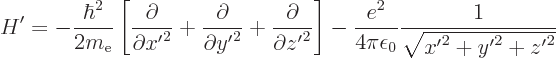
The first term is the kinetic energy operator. It is proportional to
the Laplacian operator, inside the square brackets. Standard vector
calculus says that this operator is independent of the angular
orientation of the coordinate system. So to get the corresponding
operator in the rotated  coordinate system, simply leave away
the primes. The second term is the potential energy in the field of
the proton. It is inversely proportional to the distance of the
electron from the origin. The expression for the distance from the
origin is the same in the rotated coordinate system. Once again, just
leave away the primes. The bottom line is that you cannot see a
difference between the two coordinate systems by looking at their
Hamiltonians. The expressions for the Hamiltonians are identical.
coordinate system, simply leave away
the primes. The second term is the potential energy in the field of
the proton. It is inversely proportional to the distance of the
electron from the origin. The expression for the distance from the
origin is the same in the rotated coordinate system. Once again, just
leave away the primes. The bottom line is that you cannot see a
difference between the two coordinate systems by looking at their
Hamiltonians. The expressions for the Hamiltonians are identical.
As a second example, consider the analysis of the complete hydrogen
atom as described in addendum {A.5}. The complete
atom was assumed to be in empty space; there were no external effects
on the atom included. The analysis still ignored all relativistic
effects, including the electron and proton spins. However, it did
include the motion of the proton. That meant that the kinetic energy
of the proton had to be added to the Hamiltonian. But that too is a
Laplacian, now in terms of the proton coordinates
 . Its expression too is
the same regardless of angular orientation of the coordinate system.
And in the potential energy term, the distance from the origin now
becomes the distance between electron and proton. But the formula for
the distance between two points is the same regardless of angular
orientation of the coordinate system. So once again, the expression
for the Hamiltonian does not depend on the angular orientation of the
coordinate system.
. Its expression too is
the same regardless of angular orientation of the coordinate system.
And in the potential energy term, the distance from the origin now
becomes the distance between electron and proton. But the formula for
the distance between two points is the same regardless of angular
orientation of the coordinate system. So once again, the expression
for the Hamiltonian does not depend on the angular orientation of the
coordinate system.
The equality of the Hamiltonians in the original and rotated
coordinate systems has a consequence. It leads to a mathematical
requirement for the operator of the previous subsection
that describes the effect of a coordinate system rotation on wave
functions. This operator must commute with the Hamiltonian:
That follows from examining the wave function of a system as seen in
both the original and the rotated coordinate system. There are two
ways to find the time derivative of the wave function in the rotated
coordinate system. One way is to rotate the original wave function
using to get the one in the rotated coordinate system.
Then you can apply the Hamiltonian on that. The other way is to apply
the Hamiltonian on the wave function in the original coordinate system
to find the time derivative in the original coordinate system. Then
you can use to convert that time derivative to the rotated
system. The Hamiltonian and get applied in the opposite
order, but the result must still be the same.
This observation can be inverted to define a symmetry of physics in
general:
A symmetry of physics is described by a unitary operator that
commutes with the Hamiltonian.
If an operator commutes with the Hamiltonian, then the same
Hamiltonian applies in the changed coordinate system. So there is no
physical difference in how systems evolve between the two coordinate
systems.
The qualification “unitary” means that the operator should not change the
magnitude of the wave function. The wave function should remain
normalized. It does for the transformations of interest in this note,
like rotations of the coordinate system, shifts of the coordinate
system, time shifts, and spatial coordinate inversions. All of these
transformations are unitary. Like Hermitian operators, unitary
operators have a complete set of orthonormal eigenfunctions. However,
the eigenvalues are normally not real numbers.
For those who wonder, time reversal is somewhat of a special case. To
understand the difficulty, consider first the operation “take
the complex conjugate of the wave function.” This operator
preserves the magnitude of the wave function. And it commutes with
the Hamiltonian, assuming a basic real Hamiltonian. But taking
complex conjugate is not a linear operator. For a linear operator


 . But
. But 

 . If constants come out of an operator as complex
conjugates, the operator is called “antilinear.” So taking complex conjugate is antilinear.
Another issue: a linear unitary operator preserves the inner products
between any two wave functions
. If constants come out of an operator as complex
conjugates, the operator is called “antilinear.” So taking complex conjugate is antilinear.
Another issue: a linear unitary operator preserves the inner products
between any two wave functions  and
and  . (That can
be verified by expanding the square magnitudes of
. (That can
be verified by expanding the square magnitudes of  and
and
 ). However, taking complex conjugate changes inner
products into their complex conjugates. Operators that do that are
called “antiunitary.” So taking complex conjugate is both antilinear
and antiunitary. (Of course, in normal language it is neither. The
appropriate terms would have been conjugate-linear and
conjugate-unitary. But if you got this far in this book, you know how
much chance appropriate terms have of being used in physics.)
). However, taking complex conjugate changes inner
products into their complex conjugates. Operators that do that are
called “antiunitary.” So taking complex conjugate is both antilinear
and antiunitary. (Of course, in normal language it is neither. The
appropriate terms would have been conjugate-linear and
conjugate-unitary. But if you got this far in this book, you know how
much chance appropriate terms have of being used in physics.)
Now the effect of time-reversal on wave functions turns out to be
antilinear and antiunitary too, [49, p. 76]. One simple
way to think about it is that a straightforward time reversal would
change  into
into  . Then an
additional complex conjugate will take things back to positive
energies. For the same reason you do not want to add a complex
conjugate to spatial transformations or time shifts.
. Then an
additional complex conjugate will take things back to positive
energies. For the same reason you do not want to add a complex
conjugate to spatial transformations or time shifts.
A.19.3 Derivation of the conservation law
The definition of a symmetry as an operator that commutes with the
Hamiltonian may seem abstract. But it has a less abstract
consequence. It implies that the eigenfunctions of the symmetry
operation can be taken to be also eigenfunctions of the Hamiltonian,
{D.18}. And, as chapter 7.1.4 discussed, the
eigenfunctions of the Hamiltonian are stationary. They change in time
by a mere scalar factor of magnitude 1 that does
not change their physical properties.
The fact that the eigenfunctions do not change is responsible for the
conservation law. Consider what a conservation law really means. It
means that there is some number that does not change in time. For
example, conservation of angular momentum in the -direction means
that the net angular momentum of the system in the -direction, a
number, does not change.
And if the system of particles is described by an eigenfunction of the
symmetry operator, then there is indeed a number that does not change:
the eigenvalue of that eigenfunction. The scalar factor
changes the eigenfunction, but not the eigenvalue
that would be produced by applying the symmetry operator at different
times. The eigenvalue can therefore be looked upon as a specific
value of some conserved quantity. In those terms, if the state of the
system is given by a different eigenfunction, with a different
eigenvalue, it has a different value for the conserved quantity.
The eigenvalues of a symmetry of physics describe the possible
values of a conserved quantity.
Of course, the system of particles might not be described by a single
eigenfunction of the symmetry operator. It might be a mixture of
eigenfunctions, with different eigenvalues. But that merely means
that there is quantum mechanical uncertainty in the conserved
quantity. That is just like there may be uncertainty in energy. Even
if there is uncertainty, still the mixture of eigenvalues does not
change with time. Each eigenfunction is still stationary. Therefore
the probability of getting a given value for the conserved quantity
does not change with time. In particular, neither the expectation
value of the conserved quantity, nor the amount of uncertainty in it
changes with time.
The eigenvalues of a symmetry operator may require some cleaning up.
They may not directly give the conserved quantity in the desired form.
Consider for example the eigenvalues of the rotation operator
discussed in the previous subsections. You would surely
expect a conserved quantity of a system to be a real quantity. But
the eigenvalues of are in general complex numbers.
The one thing that can be said about the eigenvalues is that they are
always of magnitude 1. Otherwise an eigenfunction would change in
magnitude during the rotation. But a function does not change in
magnitude if it is merely viewed under a different angle. And if the
eigenvalues are of magnitude 1, then the Euler formula
(2.5) implies that they can always be written in the form
where  is some real number. If the eigenvalue does not change
with time, then neither does , which is basically just
its logarithm.
is some real number. If the eigenvalue does not change
with time, then neither does , which is basically just
its logarithm.
But although is real and conserved, still it is not the
desired conserved quantity. Consider the possibility that you perform
another rotation of the axis system. Each rotation multiplies the
eigenfunction by a factor  for a total of
 . In short, if you double the angle of rotation
, you also double the value of . But it
does not make sense to say that both and
. In short, if you double the angle of rotation
, you also double the value of . But it
does not make sense to say that both and  are
conserved. If is conserved, then so is ; that
is not a second conservation law. Since is proportional to
, it can be written in the form
are
conserved. If is conserved, then so is ; that
is not a second conservation law. Since is proportional to
, it can be written in the form
where the constant of proportionality  is independent of the amount
of coordinate system rotation.
is independent of the amount
of coordinate system rotation.
The constant is the desired conserved quantity. For historical
reasons it is called the magnetic quantum number.
Unfortunately, long before quantum mechanics, classical physics had
already figured out that something was preserved. It called that
quantity the angular momentum
 . It turns
out that what classical physics defines as angular momentum is simply
a multiple of the magnetic quantum number:
. It turns
out that what classical physics defines as angular momentum is simply
a multiple of the magnetic quantum number:
So conservation of angular momentum is the same thing as conservation
of magnetic quantum number.
But the magnetic quantum number is more fundamental. Its possible
values are pure integers, unlike those of angular momentum. To see
why, note that in terms of , the eigenvalues of
are of the form
Now if you rotate the coordinate system over an angle
 , it gets back to the exact same position as it was in
before the rotation. The wave function should not change in that
case, which means that the eigenvalue must be equal to one. And that
requires that the value of is an integer. If was a fractional
number,
, it gets back to the exact same position as it was in
before the rotation. The wave function should not change in that
case, which means that the eigenvalue must be equal to one. And that
requires that the value of is an integer. If was a fractional
number,  would not be 1.
It may be interesting to see how all this works out for the two
examples mentioned in the previous subsection. The first example was the
electron in a hydrogen atom where the proton is assumed to be at rest
at the origin. Chapter 4.3 found the electron energy
eigenfunctions in the form
It is the final exponential that changes by the expected factor
 when replaces by
 .
.
The second example was the complete hydrogen atom in empty space. In
addendum {A.5}, the energy eigenfunctions were found in
the form
The first term is like before, except that it is computed with a
reduced mass
that is slightly different from the true
electron mass. The argument is now the difference in position between
the electron and the proton. It still produces a factor
when is applied. The second factor
reflects the motion of the center of gravity of the complete atom. If
the center of gravity has definite angular momentum around whatever
point is used as origin, it will produce an additional factor
 . (See addendum
{A.6} on how the energy eigenfunctions
. (See addendum
{A.6} on how the energy eigenfunctions
 can be written as spherical Bessel functions of the
first kind times spherical harmonics that have definite angular
momentum. But also see chapter 7.9 about the nasty
normalization issues with wave functions in infinite empty space.)
can be written as spherical Bessel functions of the
first kind times spherical harmonics that have definite angular
momentum. But also see chapter 7.9 about the nasty
normalization issues with wave functions in infinite empty space.)
As a final step, it is desirable to formulate a nicer operator for
angular momentum. The rotation operators are far from
perfect. One problem is that there are infinitely many of them, one
for every angle . And they are all related, a rotation
over an angle  being the same as two rotations over an angle
.
being the same as two rotations over an angle
.
If you define a rotation operator over a very small angle, call it
 , then you can approximate any other operator
by just applying sufficiently many
times. To make this approximation exact, you need to make
, then you can approximate any other operator
by just applying sufficiently many
times. To make this approximation exact, you need to make
 infinitesimally small. But when becomes
zero, would become just 1. You have lost the
nicer operator that you want by going to the extreme. The trick to
avoid this is to subtract the limiting operator 1, and in addition, to
avoid that the resulting operator then becomes zero, you must also
divide by . The nicer operator is therefore
infinitesimally small. But when becomes
zero, would become just 1. You have lost the
nicer operator that you want by going to the extreme. The trick to
avoid this is to subtract the limiting operator 1, and in addition, to
avoid that the resulting operator then becomes zero, you must also
divide by . The nicer operator is therefore
Now consider what this operator really means for a single particle
with no spin:
By definition, the final term is the partial derivative of with
respect to . So the new operator is just the operator


 !
!
You can go one better still, because the eigenvalues of the operator
just defined are
If you add a factor 
 to the operator, the eigenvalues of
the operator are going to be
to the operator, the eigenvalues of
the operator are going to be  , the quantity defined in
classical physics as the angular momentum. So you are led to define
the angular momentum operator of a single particle as:
, the quantity defined in
classical physics as the angular momentum. So you are led to define
the angular momentum operator of a single particle as:
This agrees perfectly with what chapter 4.2.2 got from
guessing that the relationship between angular and linear momentum is
the same in quantum mechanics as in classical mechanics.
The angular momentum operator of a general system can be defined
using the same scale factor:
 |
(A.76) |
The system has definite angular momentum if
Consider now what happens if the angular operator  as defined
above is applied to the wave function of a system of multiple
particles, still without spin. It produces
as defined
above is applied to the wave function of a system of multiple
particles, still without spin. It produces
The limit in the right hand side is a total derivative. According to
calculus, it can be rewritten in terms of partial derivatives to give
The scaled derivatives in the new right hand side are the orbital
angular momenta of the individual particles as defined above, so
It follows that the angular momenta of the individual particles just
add, like they do in classical physics.
Of course, even if the complete system has definite angular
momentum, the individual particles may not. A particle numbered  has definite angular momentum
  if
if
If every particle has definite momentum like that, then these
momenta directly add up to the total system momentum. At the other
extreme, if both the system and the particles have uncertain angular
momentum, then the expectation values of the momenta of the particles
still add up to that of the system.
Now that the angular momentum operator has been defined, the generator
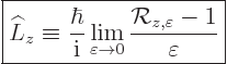
of rotations can be identified in terms of it. It turns
out to be
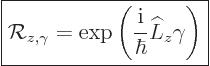 |
(A.77) |
To check that it does indeed take the form above, expand the
exponential in a Taylor series. Then apply it on an eigenfunction
with angular momentum . The effect is seen
to be to multiply the eigenfunction by the Taylor series of
 as it should. So as given above
gets all eigenfunctions right. It must therefore be correct since the
eigenfunctions are complete.
as it should. So as given above
gets all eigenfunctions right. It must therefore be correct since the
eigenfunctions are complete.
Now consider the generator of rotations in terms of the individual
particles. Since is the sum of the angular momenta of the
individual particles,
So, while the contributions of the individual particles to total
angular momentum add together, their contributions to the
generator of rotations multiply together. In particular, if a
particle has definite angular momentum , then it
contributes a factor  to .
to .
How about spin? The normal angular momentum discussed so far suggests
its true meaning. If a particle has definite spin angular
momentum in the -direction  , then presumably
the wave function changes by an additional factor
, then presumably
the wave function changes by an additional factor
 when you rotate the axis system over an angle
.
when you rotate the axis system over an angle
.
But there is something curious here. If the axis system is rotated
over an angle , it is back in its original position. So
you would expect that the wave function is also again the same as
before the rotation. And if there is just orbital angular momentum,
then that is indeed the case, because 1 as long
as is an integer, (2.5). But for fermions the spin
angular momentum  in a given direction is half-integer, and
 1. Therefore the wave function of a fermion
changes sign when the coordinate system is rotated over and is
back in its original position. That is true even if there is
uncertainty in the spin angular momentum. For example, the wave
function of a fermion with spin
1. Therefore the wave function of a fermion
changes sign when the coordinate system is rotated over and is
back in its original position. That is true even if there is
uncertainty in the spin angular momentum. For example, the wave
function of a fermion with spin  can be written as, chapter
5.5.1,
can be written as, chapter
5.5.1,
where the first term has  angular momentum in the
-direction and the second term
angular momentum in the
-direction and the second term  . Each term
changes sign under a turn of the coordinate system by .
So the complete wave function changes sign. More generally, for a
system with an odd number of fermions the wave function changes sign
when the coordinate system is rotated over . For a system
with an even number of fermions, the wave function returns to the
original value.
. Each term
changes sign under a turn of the coordinate system by .
So the complete wave function changes sign. More generally, for a
system with an odd number of fermions the wave function changes sign
when the coordinate system is rotated over . For a system
with an even number of fermions, the wave function returns to the
original value.
Now the sign of the wave function does not make a difference for the
observed physics. But it is still somewhat unsettling to see that on
the level of the wave function, nature is only the same when the
coordinate system is rotated over  instead of .
(However, it may be only a mathematical artifact. The
antisymmetrization requirement implies that the true system includes
all electrons in the universe. Presumably, the number of fermions in
the universe is infinite. That makes the question whether the number
is odd or even unanswerable. If the number of fermions does turn out
to be finite, this book will reconsider the question when people
finish counting.)
instead of .
(However, it may be only a mathematical artifact. The
antisymmetrization requirement implies that the true system includes
all electrons in the universe. Presumably, the number of fermions in
the universe is infinite. That makes the question whether the number
is odd or even unanswerable. If the number of fermions does turn out
to be finite, this book will reconsider the question when people
finish counting.)
(Some books now raise the question why the orbital angular momentum
functions could not do the same thing. Why could the quantum number
of orbital angular momentum not be half-integer too? But of course,
it is easy to see why not. If the spatial wave function would be
multiple valued, then the momentum operators would produce infinite
momentum. You would have to postulate arbitrarily that the
derivatives of the wave function at a point only involve wave function
values of a single branch. Half-integer spin does not have the same
problem; for a given orientation of the coordinate system, the
opposite wave function is not accessible by merely changing position.)
A.19.4 Other symmetries
The previous subsections derived conservation of angular momentum from
the symmetry of physics with respect to rotations. Similar arguments
may be used to derive other conservation laws. This subsection
briefly outlines how.
Conservation of linear momentum can be derived from the symmetry of
physics with respect to translations. The derivation is completely
analogous to the angular momentum case. The translation operator
 shifts the coordinate system over a distance
  in
the -direction. Its eigenvalues are of the form
in
the -direction. Its eigenvalues are of the form
where  is a real number, independent of the amount of translation
, that is called the wave number. Following the same
arguments as for angular momentum, is a preserved quantity. In
classical physics not , but
is a real number, independent of the amount of translation
, that is called the wave number. Following the same
arguments as for angular momentum, is a preserved quantity. In
classical physics not , but 
 is
defined as the conserved quantity. To get the operator for this
quantity, form the operator
is
defined as the conserved quantity. To get the operator for this
quantity, form the operator
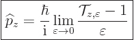 |
(A.78) |
For a single particle, this becomes the usual linear momentum operator

 . For multiple particles, the
linear momenta add up.
. For multiple particles, the
linear momenta add up.
It may again be interesting to see how that works out for the two
example systems introduced earlier. The first example was the
electron in a hydrogen atom. In that example it is assumed that
the proton is fixed at the origin. The energy eigenfunctions for
the electron then were of the form
with  the position of the electron. Shifting the coordinate
system for this solution means replacing by
the position of the electron. Shifting the coordinate
system for this solution means replacing by  .
That shifts the position of the electron without changing the position
of the proton. The physics is not the same after such a shift.
Correspondingly, the eigenfunctions do not change by a factor of the
form
.
That shifts the position of the electron without changing the position
of the proton. The physics is not the same after such a shift.
Correspondingly, the eigenfunctions do not change by a factor of the
form  under the shift. Just looking at the ground
state,
under the shift. Just looking at the ground
state,
is enough to see that. An electron around a stationary proton does
not have definite linear momentum. In other words, the linear
momentum of the electron is not conserved.
However, the physics of the complete hydrogen atom as described in
addendum {A.5} is independent of coordinate shifts. A
suitable choice of energy eigenfunctions in this context is
where  is a constant wave number vector. The first factor does
not change under coordinate shifts because the vector
is a constant wave number vector. The first factor does
not change under coordinate shifts because the vector
 from proton to electron does not. The exponential
changes by the expected factor because the position
from proton to electron does not. The exponential
changes by the expected factor because the position
 of the center of gravity of the atom changes by an
amount in the -direction.
of the center of gravity of the atom changes by an
amount in the -direction.
The derivation of linear momentum can be extended to conduction
electrons in crystalline solids. In that case, the physics of the
conduction electrons is unchanged if the coordinate system is
translated over a crystal period . (This assumes that the
-axis is chosen along one of the primitive vectors of the crystal
structure.) The eigenvalues are still of the form
. However, unlike for linear momentum, the
translation must be the crystal period, or an integer multiple of
it. Therefore, the operator  is not useful; the symmetry does
not continue to apply in the limit
is not useful; the symmetry does
not continue to apply in the limit  .
.
The conserved quantity in this case is just the
eigenvalue of . It is not possible from that
eigenvalue to uniquely determine a value of and the
corresponding crystal momentum . Values of
that differ by a whole multiple of produce the same
eigenvalue. But Bloch waves have the same indeterminacy in their
value of anyway. In fact, Bloch waves are eigenfunctions of
as well as energy eigenfunctions.
One consequence of the indeterminacy in is an increased number
of possible electromagnetic transitions. Typical electromagnetic
radiation has a wave length that is large compared to the atomic
spacing. Essentially the electromagnetic field is the same from one
atom to the next. That means that it has negligible crystal momentum,
using the smallest of the possible values of  as measure.
Therefore the radiation cannot change the conserved eigenvalue
. But it can still produce electron transitions
between two Bloch waves that have been assigned different values
in some
as measure.
Therefore the radiation cannot change the conserved eigenvalue
. But it can still produce electron transitions
between two Bloch waves that have been assigned different values
in some extended zone scheme,
chapter 6.22.4.
As long as the two values differ by a whole multiple of
, the actual eigenvalue does not
change. In that case there is no violation of the conservation law in
the transition. The ambiguity in values may be eliminated by
switching to a reduced zone scheme
description,
chapter 6.22.4.
The time shift operator  shifts the time coordinate over an
interval
shifts the time coordinate over an
interval  . In empty space, its eigenfunctions are exactly
the energy eigenfunctions. Its eigenvalues are of the form
. In empty space, its eigenfunctions are exactly
the energy eigenfunctions. Its eigenvalues are of the form
where classical physics defines  as the energy
  .
The energy operator can be defined correspondingly, and is simply the
Hamiltonian:
.
The energy operator can be defined correspondingly, and is simply the
Hamiltonian:
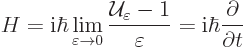 |
(A.79) |
In other words, we have reasoned in a circle and rederived the
Schrödinger equation from time shift symmetry. But you could
generalize the reasoning to the motion of particles in an external
field that varies periodically in time.
Usually, nature is not just symmetric under rotating or translating
it, but also under mirroring it. A transformation that creates a
mirror image of a given system is called a parity transformation. The
mathematically cleanest way to do it is to invert the direction of
each of the three Cartesian axes. That is called spatial inversion.
Physically it is equivalent to mirroring the system using some mirror
passing through the origin, and then rotating the system
180 around the axis normal to the mirror.
(In a strictly two-dimensional system, spatial inversion does not work,
since the rotation would take the system into the third dimension. In
that case, mirroring can be achieved by replacing just  by
in some suitably chosen
by
in some suitably chosen  -coordinate system. Subsequently
replacing
-coordinate system. Subsequently
replacing  by would amount to a second mirroring that would
restore a nonmirror image. In those terms, in three dimensions it is
replacing by that produces the final mirror image in
spatial inversion.)
by would amount to a second mirroring that would
restore a nonmirror image. In those terms, in three dimensions it is
replacing by that produces the final mirror image in
spatial inversion.)
The analysis of the conservation law corresponding to spatial
inversion proceeds much like the one for angular momentum. One
difference is that applying the spatial inversion operator a second
time turns back into the original . Then the
wave function is again the same. In other words, applying spatial
inversion twice multiplies wave functions by 1. It follows that the
square of every eigenvalue is 1. And if the square of an eigenvalues
is 1, then the eigenvalue itself must be either 1 or 1. In the same
notation as used for angular momentum, the eigenvalues of the spatial
inversion operator can therefore be written as
 |
(A.80) |
where  must be integer. However, it is pointless to give an
actual value for ; the only thing that makes a difference
for the eigenvalue is whether is even or odd. Therefore, parity
is simply called
must be integer. However, it is pointless to give an
actual value for ; the only thing that makes a difference
for the eigenvalue is whether is even or odd. Therefore, parity
is simply called odd” or “minus one
or
negative
if the eigenvalue is 1, and
even” or “one
or
positive
if the eigenvalue is 1.
In a system, the  parity eigenvalues of the individual particles
multiply together. That is just like how the eigenvalues of the
generator of rotation multiply together for angular
momentum. Any particle with even parity has no effect on the system
parity; it multiples the total eigenvalue by 1. On the other hand,
each particle with odd parity flips over the total parity from odd to
even or vice-versa; it multiplies the total eigenvalue by 1.
Particles can also have intrinsic parity. However, there is no
half-integer parity like there is half-integer spin.
parity eigenvalues of the individual particles
multiply together. That is just like how the eigenvalues of the
generator of rotation multiply together for angular
momentum. Any particle with even parity has no effect on the system
parity; it multiples the total eigenvalue by 1. On the other hand,
each particle with odd parity flips over the total parity from odd to
even or vice-versa; it multiplies the total eigenvalue by 1.
Particles can also have intrinsic parity. However, there is no
half-integer parity like there is half-integer spin.
A.19.5 A gauge symmetry and conservation of charge
Modern quantum theories are build upon so-called “gauge
symmetries.” This subsection gives a simple introduction to
some of the ideas.
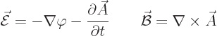
Consider classical electrostatics. The force on charged particles is
the product of the charge of the particle times the so-called electric
field  . Basic physics says that the electric field is
minus the derivative of a potential
. Basic physics says that the electric field is
minus the derivative of a potential  . The potential
is commonly known as the
. The potential
is commonly known as the voltage
in
electrical applications. Now it too has a symmetry: adding some
arbitrary constant, call it  , to does not make a
difference. Only differences in voltage can be observed
physically. That is a very simple example of a gauge symmetry, a
symmetry in an unobservable field, here the potential .
, to does not make a
difference. Only differences in voltage can be observed
physically. That is a very simple example of a gauge symmetry, a
symmetry in an unobservable field, here the potential .
Note that this symmetry does not involve the gauges used to measure
voltages in any way. Instead it is a reference point symmetry; it
does not make a difference what voltage you want to declare to be
zero. It is conventional to take the earth as the reference voltage,
but that is a completely arbitrary choice. So the term “gauge
symmetry” is misleading, like many other terms in physics. A
symmetry in a unobservable quantity should of course simply have been
called an unobservable symmetry.
There is a relationship between this gauge symmetry in and
charge conservation. Suppose that, say, a few photons create an
electron and an antineutrino. That can satisfy conservation of
angular momentum and of lepton number, but it would violate charge
conservation. Photons have no charge, and neither have neutrinos. So
the negative charge  of the electron would appear out of nothing.
But so what? Photons can create electron-positron pairs, so why not
electron-antineutrino pairs?
of the electron would appear out of nothing.
But so what? Photons can create electron-positron pairs, so why not
electron-antineutrino pairs?
The problem is that in electrostatics an electron has an electrostatic
energy  . Therefore the photons would need to provide
not just the rest mass and kinetic energy for the electron and
antineutrino, but also an additional electrostatic energy
. That additional energy could be determined from
comparing the energy of the photons against that of the
electron-antineutrino pair. And that would mean that the value of
at the point of pair creation has been determined. Not just
a difference in values between different points. And that
would mean that the value of the constant would be fixed. So
nature would not really have the gauge symmetry that a constant in the
potential is arbitrary.
. Therefore the photons would need to provide
not just the rest mass and kinetic energy for the electron and
antineutrino, but also an additional electrostatic energy
. That additional energy could be determined from
comparing the energy of the photons against that of the
electron-antineutrino pair. And that would mean that the value of
at the point of pair creation has been determined. Not just
a difference in values between different points. And that
would mean that the value of the constant would be fixed. So
nature would not really have the gauge symmetry that a constant in the
potential is arbitrary.
Conversely, if the gauge symmetry of the potential is fundamental to
nature, creation of lone charges must be impossible. Each negatively
charged electron that is created must be accompanied by a positively
charged particle so that the net charge that is created is zero. In
electron-positron pair creation, the positive charge  of the
positron makes the net charge that is created zero. Similarly, in
beta decay, an uncharged neutron creates an electron-antineutrino pair
with charge , but also a proton with charge .
of the
positron makes the net charge that is created zero. Similarly, in
beta decay, an uncharged neutron creates an electron-antineutrino pair
with charge , but also a proton with charge .
You might of course wonder whether an electrostatic energy
contribution is really needed to create an electron. It
is because of energy conservation. Otherwise there would be a problem
if an electron-antineutrino pair was created at a location P and
disintegrated again at a different location Q. The electron would
pick up a kinetic energy  while
traveling from P to Q. Without electrostatic contributions to the
electron creation and annihilation energies, that kinetic energy would
make the photons produced by the pair annihilation more energetic than
those destroyed in the pair creation. So the complete process would
create additional photon energy out of nothing.
while
traveling from P to Q. Without electrostatic contributions to the
electron creation and annihilation energies, that kinetic energy would
make the photons produced by the pair annihilation more energetic than
those destroyed in the pair creation. So the complete process would
create additional photon energy out of nothing.
The gauge symmetry takes on a much more profound meaning in quantum
mechanics. One reason is that the Hamiltonian is based on the
potential, not on the electric field itself. To appreciate the full
impact, consider electrodynamics instead of just electrostatics. In
electrodynamics, a charged particle does not just experience an
electric field but also a magnetic field  . There is
a corresponding additional so-called
. There is
a corresponding additional so-called vector potential
 in addition to the scalar potential . The
relation between these potentials and the electric and magnetic fields
is given by, chapter 13.1:
in addition to the scalar potential . The
relation between these potentials and the electric and magnetic fields
is given by, chapter 13.1:
Here  , nabla, is the differential operator of vector
calculus (calculus III in the U.S. system):
, nabla, is the differential operator of vector
calculus (calculus III in the U.S. system):
The gauge property now becomes more general. The constant that
can be added to in electrostatics no longer needs to be
constant. Instead, it can be taken to be the time-derivative of any
arbitrary function  . However, the gradient of
this function must also be subtracted from . In
particular, the potentials
. However, the gradient of
this function must also be subtracted from . In
particular, the potentials
produce the exact same electric and magnetic fields as and
. So they are physically equivalent. They produce the
same observable motion.
However, the wave function computed using the potentials  and
and
 is different from the one computed using and
. The reason is that the Hamiltonian uses the potentials
rather than the electric and magnetic fields. Ignoring spin, the
Hamiltonian of an electron in an electromagnetic field is, chapter
13.1:
is different from the one computed using and
. The reason is that the Hamiltonian uses the potentials
rather than the electric and magnetic fields. Ignoring spin, the
Hamiltonian of an electron in an electromagnetic field is, chapter
13.1:
It can be seen by crunching it out that if satisfies the Schrödinger
equation in which the Hamiltonian is formed with and
, then
 |
(A.81) |
satisfies the one in which is formed with and
.
To understand what a stunning result that is, recall the physical
interpretation of the wave function. According to Born, the square
magnitude of the wave function  determines the probability
per unit volume of finding the electron at a given location. But the
wave function is a complex number; it can always be written in the
form
determines the probability
per unit volume of finding the electron at a given location. But the
wave function is a complex number; it can always be written in the
form
where is a real quantity corresponding to a phase angle.
This angle is not directly observable; it drops out of the magnitude
of the wave function. And the gauge property above shows that not
only is not observable, it can be anything. For, the
function  can change by a completely arbitrary amount
  and it remains a
solution of the Schrödinger equation. The only variables that change are
the equally unobservable potentials and .
and it remains a
solution of the Schrödinger equation. The only variables that change are
the equally unobservable potentials and .
As noted earlier, a symmetry means that you can do something and it
does not make a difference. Since can be chosen completely
arbitrary, varying with both location and time, this is a very strong
symmetry. Zee writes, (Quantum Field Theory in a Nutshell, 2003,
p. 135): "The modern philosophy is to look at [the equations of
quantum electrodynamics] as a result of [the gauge symmetry above].
If we want to construct a gauge-invariant relativistic field theory
involving a spin and a spin 1 field, then we are forced to
quantum electrodynamics."
Geometrically, a complex number like the wave function can be shown in
a two-dimensional complex plane in which the real and imaginary parts
of the number form the axes. Multiplying the number by a factor
 corresponds to rotating it over an angle
around the origin in that plane. In those terms, the
wave function can be rotated over an arbitrary, varying, angle in the
complex plane and it still satisfies the Schrödinger equation.
corresponds to rotating it over an angle
around the origin in that plane. In those terms, the
wave function can be rotated over an arbitrary, varying, angle in the
complex plane and it still satisfies the Schrödinger equation.
For a relatively accessible derivation how the gauge invariance
produces quantum electrodynamics, see [24, pp. 358ff].
To make some sense out of it, chapter 1.2.5 gives a brief
inroduction to relativistic index notation, chapter 12.12 to
the Dirac equation and its matrices, addendum {A.1} to
Lagrangians, and {A.21} to photon wave functions. The
 are derivatives of this wave function,
[24, p. 239].
are derivatives of this wave function,
[24, p. 239].
A.19.6 Reservations about time shift symmetry
It is not quite obvious that the evolution of a physical system in
empty space is the same regardless of the time that it is started. It
is certainly not as obvious as the assumption that changes in spatial
position do not make a difference. Cosmology does not show any
evidence for a fundamental difference between different locations in
space. For each spatial location, others just like it seem to exist
elsewhere. But different cosmological times do show a major physical
distinction. They differ in how much later they are than the time of
the creation of the universe as we know it. The universe is
expanding. Spatial distances between galaxies are increasing. It is
believed with quite a lot of confidence that the universe started out
extremely concentrated and hot at a “Big Bang” about 15 billion years ago.
Consider the cosmic background radiation. It has cooled down greatly
since the universe became transparent to it. The expansion stretched
the wave length of the photons of the radiation. That made them less
energetic. You can look upon that as a violation of energy
conservation due to the expansion of the universe.
Alternatively, you could explain the discrepancy away by assuming that
the missing energy goes into potential energy of expansion of the
universe. However, whether this potential energy
is
anything better than a different name for “energy that got
lost” is another question. Potential energy is normally energy
that is lost but can be fully recovered. The potential energy of
expansion of the universe cannot be recovered. At least not on a
global scale. You cannot stop the expansion of the universe.
And a lack of exact energy conservation may not be such a bad thing
for physical theories. Failure of energy conservation in the early
universe could provide a possible way of explaining how the universe
got all that energy in the first place.
In any case, for practical purposes nontrivial effects of time shifts
seem to be negligible in the current universe. When astronomy looks
at far-away clusters of galaxies, it sees them as they were billions
of years ago. That is because the light that they emit takes billions
of years to reach us. And while these galaxies look different from
the current ones nearby, there is no evident difference in their basic
laws of physics. Also, gravity is an extremely small effect in most
other physics. And normal time variations are negligible compared to
the age of the universe. Despite the Big Bang, conservation of energy
remains one of the pillars on which physics is build.

![\begin{displaymath}
\L _z \Psi = \frac{\hbar}{{\rm i}}
\left[
\frac{\partial...
..._1} +
\frac{\partial}{\partial\phi_2} +
\ldots
\right] \Psi
\end{displaymath}](img4230.gif)