| Quantum Mechanics for Engineers |
|
© Leon van Dommelen |
|
D.58 The canonical probability distribution
This note deduces the canonical probability distribution. Since the
derivations in typical textbooks seem crazily convoluted and the made
assumptions not at all as self-evident as the authors suggest, a more
mathematical approach will be followed here.
Consider a big system consisting of many smaller subsystems
 with a given total energy
  . Call the combined
system the collective. Following the same reasoning as in derivation
{D.57} for two systems, the thermodynamically stable
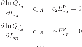
equilibrium state has shelf occupation numbers of the subsystems
satisfying
where  is a shorthand for 1/
 .
.
An individual system, take  as the example, no longer has an
individual energy that is for certain. Only the collective has that.
That means that when
  is taken out of the collective, its shelf
occupation numbers will have to be described in terms of
probabilities. There will still be an expectation value for the
energy of the system, but system energy eigenfunctions
  with somewhat different energy
  can no longer be excluded
with certainty. However, still assume, following the fundamental
assumption of quantum statistics, {N.23}, that the
physical differences between the system energy eigenfunctions do not
make (enough of) a difference to affect which ones are likely or not.
So, the probability
  of a system eigenfunction
  will be assumed to depend only on its energy
  :
:

where  is some as yet unknown function.
For the isolated example system  , the question is now no
longer “What shelf numbers have the most
eigenfunctions?” but “What shelf numbers have the
highest probability?” Note that all system eigenfunctions
 for a given set of shelf numbers
  have the
same system energy

 . Therefore, the probability of a
given set of shelf numbers
  will be the number of
eigenfunctions with those shelf numbers times the probability of each
individual eigenfunction:
Mathematically, the function whose partial derivatives must be zero to
find the most probable shelf numbers is
The maximum is now to be found for the shelf number probabilities,
not their eigenfunction counts, and there is no longer a constraint on
energy.
Substituting 

 , taking apart the logarithm,
and differentiating, produces
That is exactly like the equation for the shelf numbers of system  when it was part of the collective, except that the derivative of the
as yet unknown function
  takes the place of
 , i.e.
  1/
1/ . It follows that the two
must be the same, because the shelf numbers cannot change when the
system
  is taken out of the collective it is in thermal equilibrium
with. For one, the net energy would change if that happened, and
energy is conserved.
It follows that 


 1
1
 at least in the vicinity of the most probable energy
 . Hence in the vicinity of that energy
which is the canonical probability. Note that the given derivation
only ensures it to be true in the vicinity of the most probable
energy. Nothing says it gives the correct probability for, say, the
ground state energy. But then the question becomes “What
difference does it make?” Suppose the ground state has a
probability of 0. followed by only 100 zeros instead of the
predicted 200 zeros? What would change in the price of eggs?
Note that the canonical probability is self-consistent: if two systems
at the same temperature are combined, the probabilities of the
combined eigenfunctions multiply, as in
That is still the correct expression for the combined system, since
its energy is the sum of those of the two separate systems. Also for
the partition functions
![]()
![]() .
.
![]()
![]()
![]()
![]()
![]()
![]()
![]() :
:![]() ,
,![]()
![]()
![]()
![]()
![]() .
.![]()

![]()
![]()
![]() ,
,
![]()
![]()
![]()
![]()
![]() 1
1![]()
![]()
![]() .
.