Next: The backward heat
Up: The heat equation.
Previous: About evolution equations.
The fact that the heat equation is an evolution equation simplifies
how the solution to the heat conduction problem can be obtained
numerically. We will postpone a complete discussion to a later time,
but some issues in a typical computation are already self evident.
For example, according to what we said above, to solve the heat
conduction problem completely requires the determination of the
temperature at all points in the strip in the x,t-plane
figure 2. That would be an infinity of points and
unknowns, something a digital computer cannot deal with. To make the
number of unknowns finite, the points at which to find the temperature
can be artificially restricted to a finite set by only including a
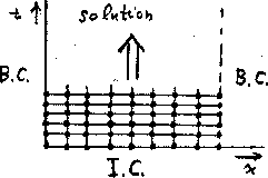
mesh, or grid, of discrete points as shown in
figure 4. (Of course, some approximations will need
to be made to allow us to ignore the points that were ommitted, which
could be done, for example, using a finite difference, nodal finite
element, or spectral collocation procedure.)
Figure 4:
Typical numerical solution of the heat equation.
 |
Using a mesh, solving the heat conduction problem reduces finding the
temperature values at a finite number of points. When a finer mesh,
with more mesh points, is used, the accuracy will be higher, but so
will the computational effort. Fortunately, for an evolution equation we
do not have to try to find all these values at the same time. The
values at the initial time plane in figure 4 are
already known from the given initial condition (5).
Now, if we look at the next higher time level, the temperature values
can depend on the known initial values and the boundary conditions,
but they cannot depend on the later time levels. As a result, we can
find the temperature values at this second time level without worrying
about the later ones. This makes the number of unknowns we have to
deal with at once much smaller, which is usually a big advantage.
After we have found the second time level, we can proceed with the
third, and so on. In other words, we ``march'' the solution forward
in time.
Next: The backward heat
Up: The heat equation.
Previous: About evolution equations.
