EML 3002L M.E. Tools Lab 11/07/19
MATLAB Exam 2 Van Dommelen 12:30-1:45 pm

NO CELL PHONES, HEADPHONES/BUDS, NO CALCULATORS. SAVE FREQUENTLY. SAVE BEFORE PUBLISHING!!!

ONLY MATLAB MAY BE ACTIVE ON YOUR COMPUTER. Acrobat may only be open at the end, when you are ready except for publishing and actively looking at q1.pdf, q2.pdf, or q3.pdf with it.

VARIABLE NAMES MUST BE APPROPRIATE AND CLEARLY SHOW WHAT VARIABLE IT IS OR A 50% CREDIT REDUCTION IS APPLIED. USE THE SAME NAMES AS IN THE QUESTION. All results must have an appropriate understandable name, not ans.

After translation into mathematics, only MATLAB may be used to solve the full problem as posed. Use the appropriate procedures as covered in the lectures.

Open notes: print-outs of lectures and homeworks allowed. You can also use your own homework .m files.

1. Set $n$, n, to 4. Then initialize a square matrix $A$, A, of size $n\times{}n$ and use a nested for loop to set A(i,j) to i*j for all values of i and j from 1 to n. This “multiplication matrix” should then look like
   
   $$A = \left( \begin{array}{cccc} 1 & 2 & 3 & 4 \\ 2 & 4 ... ...\\ 3 & 6 & 9 & 12 \\ 4 & 8 & 12 & 16 \end{array} \right)$$
   
   
   However, your code should work for any value of $n$, not just 4.

   If you cannot get this to work, behind your feeble attempts, just set $A$ manually to the above values to do the rest.

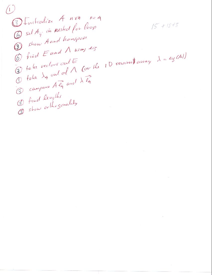
   Show both A and its transpose to verify that A is symmetric.

   Now let MATLAB find the eigenvalues and eigenvectors of this matrix. Then put the last two eigenvectors $\vec{e}_3$ and $\vec{e}_4$ in separate one-dimensional arrays called eVec3 and eVec4 and put the last eigenvalue $\lambda_4$ in a scalar variable lam4. Then use eVec4 and lam4 to verify directly that indeed $A\vec{e}_4=\lambda_4\vec{e}_4$. Also verify that the lengths of both eVec3 and eVec4 are one, and that eVec3 is orthogonal to eVec4.

   Solution Grading

2. Using the Symbolic Math Toolbox:
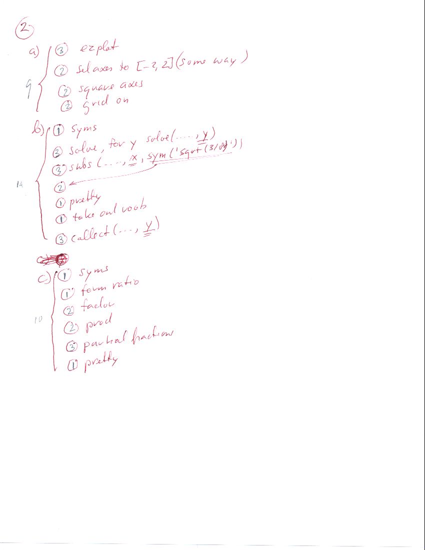
   1. Use the appropriate ez... function to plot the Folium of Descartes
      
      $$x^3 + y^3 - 3xy = 0$$
      
      
      Restrict $x$ and $y$ to the range from $-$2 to 2. Use a square axis system and a grid.

   2. The equation for the lemniscate of Bernoulli is
      
      $$(x^2+y^2)^2=x^2-y^2$$
      
      
      Solve this equation symbolically to give $y$ in terms of $x$. Then substitute the value $x=\sqrt{3/8}$ into the solution and see what you get for $y$. Show the pretty version of this solution also. You should get 4 roots, but only two of these roots are real. Show the two real roots separately as symbolic expressions y1 and y2. Finally, collect the coefficients of the powers of $y$ in the symbolic expression
      
      $$(x^2+y^2)^2-x^2+y^2$$
      
      
      together to see why the Toolbox solves the expression so easily: it is a quadratic equation if you take $y^2$ as the unknown!

   3. Define a symbolic ratio ratSym as
      
      $$\frac{s^3-2s^2-5s+6}{s^4-16}$$
      
      
      Then show this ratio as a single factored ratio. Also show the partial fraction expansion of the ratio. Give a pretty version of the latter.

   Solution Grading

3. Consider heat conduction in a square plate that extends horizontally from $x=0$ to $x=1$ and vertically from $y=0$ to $y=1$. Define an array xVals to contain $n=11$ equally spaced $x$-values from 0 to 1 and an array yVals to contain $m=11$ equally spaced $y$-values from 0 to 1. (While we are taking $m=n=11$, your program should continue to work correctly if the values of $m$ and $n$ are changed.)

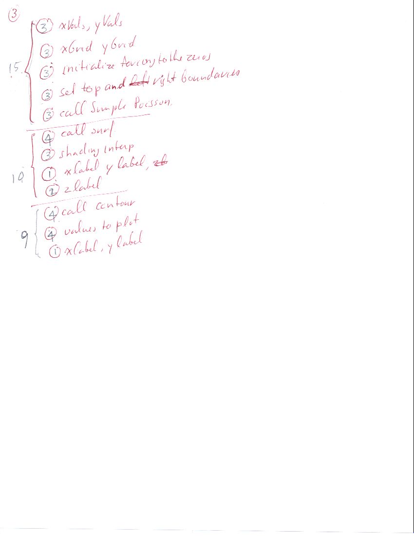
   Then define a two-dimensional grid for the plate in which the grid points have these $x$ and $y$-values. Also define an array forcing for the grid points that is zero for the grid points in the interior of the plate. For the grid points on the boundaries of the plate, array forcing should have the given temperatures on the boundary: For the left hand and bottom boundaries the temperature is given to be zero, but on the right hand boundary it is $y$ and on the top boundary it is $x^2$. Put that in array forcing. Then use array forcing in function SimplePoisson to create the temperature values TGrid at all the grid points. (Ignore the warning about CONDEST.)

   (Note: If you cannot get TGrid right, behind your feeble attempts, put the code

       xGrid=zeros(m,n); yGrid=zeros(m,n); TGrid=zeros(m,n);
       for i=1:m; for j=1:n
           xGrid(i,j)=xVals(j); yGrid(i,j)=yVals(i);
           TGrid(i,j)=xVals(j)^2*yVals(i);
       end; end

   which will produce a fake TGrid good enough for doing the rest of this question.)

   Plot the obtained temperature distribution as a surface with smoothly varying shading. Label all three axes, the temperature axis as Temperature.

   Also plot the isotherms (lines of constant temperature) in the $x,y$ plane. In particular, plot the lines where the temperature is 0.1, 0.2, ..., and 0.9. Label the axes.

   Use double percent lines and/or figure numbers to ensure that both plots end up in the published pdf file.

   Solution Grading