EML 3002L M.E. Tools Lab 10/10/17
Matlab Exam 1 Van Dommelen 12:30-1:45 pm
NO CELL PHONES. NO HEADPHONES/BUDS. NO CALCULATORS. You may only
have a pen or pencil with you and use this exam sheet for scratch
paper. ONLY MATLAB MAY BE ACTIVE ON YOUR COMPUTER.
SAVE FREQUENTLY. A CRASH IS NO EXCUSE FOR ANYTHING. SAVE BEFORE
PUBLISHING!!! REMAIN SEATED AT ALL TIMES.
After translation into mathematics, only Matlab may be used to
solve the full problem as posed. Use the appropriate procedures
as covered in the lectures. Use appropriate variable names that can
be clearly understood by the grader. Use appropriate comments.
Acrobat may only be open at the end, when you are ready except for
publishing and actively looking at main.pdf with it.
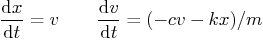
- Plot the two functions
 and
and  in the same graph
from 0 to 2. Then find the positive root
in the same graph
from 0 to 2. Then find the positive root  where the two
functions are equal using the search interval method. The values of
the end points of the interval you use must be integers, and you
must check the end point function values for acceptability. Explain
in the comments why your end values are acceptable. Print the root
out formatted by Matlab as
where the two
functions are equal using the search interval method. The values of
the end points of the interval you use must be integers, and you
must check the end point function values for acceptability. Explain
in the comments why your end values are acceptable. Print the root
out formatted by Matlab as The root is: *.123456
,
i.e. 6 digits behind the decimal point and Matlab's default number
of print positions before the point. No hard-coding the number
allowed.
Warning: Do not forget the point before the squaring operator in
.
Grading
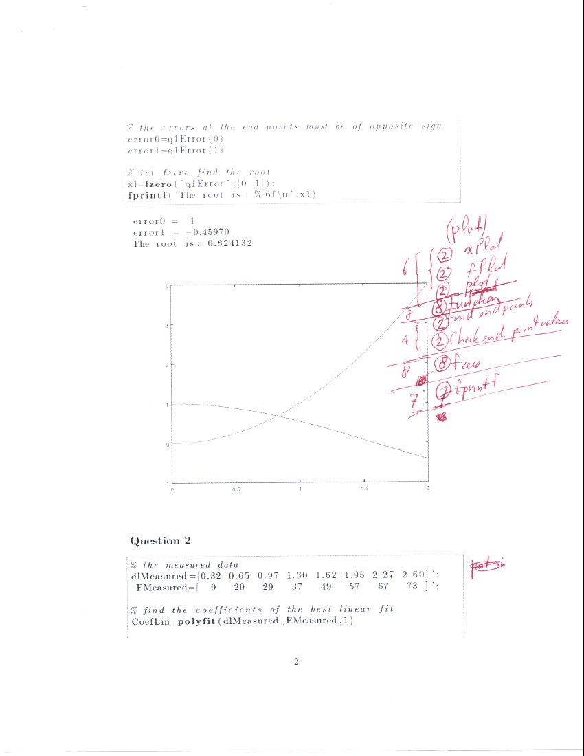
- Consider the following measured data on the elongation
 of a
linear spring versus the force it supports:
of a
linear spring versus the force it supports:
 in: 0.32 in: 0.32 |
0.65 |
0.97 |
1.30 |
1.62 |
1.95 |
2.27 |
2.60 |
|
 lbf: 9 lbf: 9 |
20 |
29 |
37 |
49 |
57 |
67 |
73 |
|
- Fit a straight line to the given data using linear regression.
Use it to print the best value of the force at an elongation of
1.5.
- Plot both the data, as circles, and the straight line
representation, as a continuous line, in the same graph with the
vertical axis from 0 to 90, horizontal from 0 to 3. Title it
Best Force/Displacement Approximation
, and use
axes labels dl inch” and “F lbf
.
Prevent the legend from crossing the line; put it in an empty spot
in the plot.
Grading
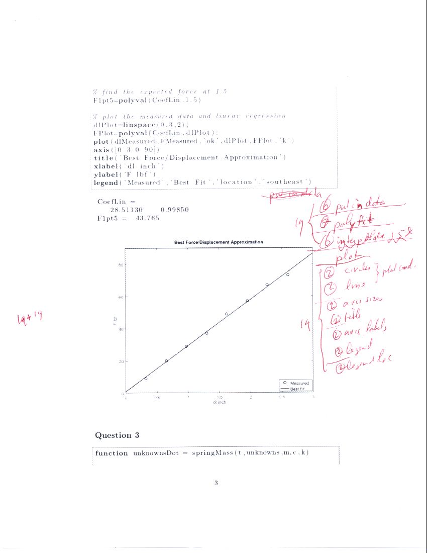
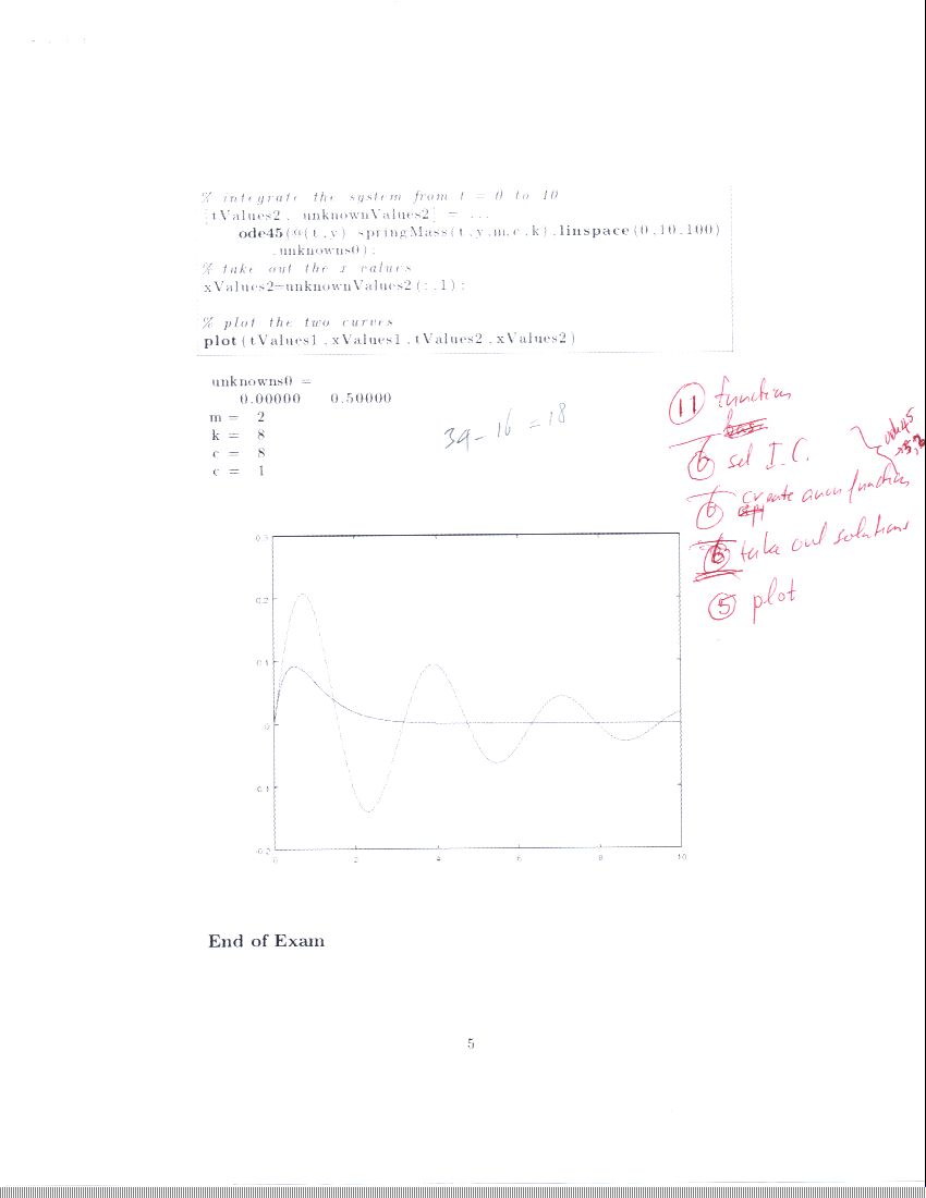
- Each corner of a car may be modeled as a mass attached to a
spring and a damper (shock absorber). That produces the simplest
vibrating system in mechanical engineering (and physics in general),
the damped linear spring-mass system. Its vertical motion is
described by
| |  |
|
| |
(1) |
where  is the vertical position of the corner measured from
equilibrium,
is the vertical position of the corner measured from
equilibrium,  its vertical velocity,
  the effective mass,
  the damping constant, and
  the spring constant. Assume that
 and
and  and that initially, the vertical position is
normal, so zero, but that there is a vertical velocity
and that initially, the vertical position is
normal, so zero, but that there is a vertical velocity  due
to hitting a speed bump. Find the position for times
due
to hitting a speed bump. Find the position for times
 for two cases; (a)
  , “good
shocks”, and (b)
, “good
shocks”, and (b)  ,
, bad shocks
. Plot the
two curves in the same graph. Special requirements: use the same
function file to do both cases (a) and (b). Call your function file
'springMass.m'. Specify the time range as about 100 points from 0
to 10, not just [0 10], which would make the plot look
horrible.
Grading
Solutions without credit distribution.
Solutions with credit distribution.